Local Area Networks (LANs)

Rita Mitra; Glenn Brown; Melanie Huffman; Hongyi Zhu

13 Local Area Networks (LANs)

Chapter Objectives

Outline the major features and functions of a local area network (LAN).
Compare different network topologies, such as bus, ring, star, tree, and mesh.
Evaluate the network efficiency of a LAN in terms of fairness, node buffers, node capacity, and other features.
Distinguish between deterministic and stochastic medium access control (MAC) algorithms.
Compare static and dynamic allocation schemes in the access of multiple devices to a shared communication channel.
Describe the applicability of different MAC algorithms, such as FDMA, TDMA, CSMA/CA, and CSMA/CD for various LAN scenarios.
Explain techniques for congestion control and for avoiding congestion collapse, such as backoff algorithms, window policy, discarding policy, acknowledgment policy, or admission policy.
Outline the major features and functions of a virtual local area network (VLAN).

Local Area Networks (LANs)

Shahabalikhattak. English: This File Represents the Structure and Frame Fields of Ethernet Frame. 6 Apr. 2019. Own work, Wikimedia Commons, https://commons.wikimedia.org/wiki/File:Ethernet_II_Frame_Structure.png.

One of the challenges of LAN communication is how to handle collisions, which occur when two or more devices try to send data at the same time on the same medium. Collisions can cause data loss and reduce the network efficiency. We will discuss techniques to avoid or resolve collisions later in this chapter. First, let’s look at common network topologies.

Network Topologies

The first and more important resource inside a network is the link bandwidth. Link bandwidth needs to be shared between different users when several hosts are attached to the same physical link in a LAN. Consider for example a network with five hosts. Any of these hosts needs to be able to exchange information with any of the other hosts using some sort of topological design.

Network topology is the arrangement of the devices and links that make up a network. A topology can be defined by its physical design, which means how the devices are actually connected by cables or wireless signals, or by its logical design, which refers to how data is transmitted, or routed, across the network between devices. Different types of network topologies have different advantages and disadvantages in terms of performance, reliability, cost, and scalability. Below, we discuss the major topologies of a LAN network.

Bus

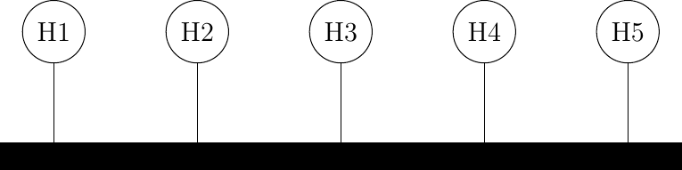
In this topology, each device is connected to a single cable that runs through the entire network. The cable acts as a shared medium for all the devices on the network. This topology is cheap and easy to install, and requires less cable than other topologies. However, it also has some disadvantages, such as low security, low speed, high possibility of collisions, and difficulty in troubleshooting.

The bus network, also used inside computers to connect different extension cards, is one in which all hosts are attached to a shared medium, which is usually a cable through a single interface. When one host sends an electrical signal on the bus, the signal is received by all hosts attached to the bus. A drawback of bus-based networks is that if the bus is physically cut, then the network is split into two isolated networks. For this reason, bus-based networks are sometimes considered to be difficult to operate and maintain, especially when the cable is long and there are many places where it can break. The bus-based topology was used in early Ethernet networks.

A network organized as a bus

Star

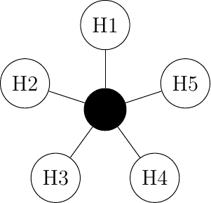
In this topology, each device is connected to a central device, such as a switch or a hub, by a single cable. The central device acts as a point of connection and communication for all the devices on the network. This topology is easy to install and manage, and allows easy addition or removal of devices. However, it also has some drawbacks, such as high dependency on the central device, which can be a single point of failure, and high cost of cabling.

In star networks, hosts have a single physical interface with one physical link between each host and the center of the star. The node at the center of the star can be either a piece of equipment that amplifies an electrical signal, or an active device, such as a piece of equipment that understands the format of the messages exchanged through the network. As noted, the failure of the central node implies the failure of the network. However, if one physical link fails (e.g. because the cable has been cut), then only one node is disconnected from the network. In practice, star-shaped networks are easier to operate and maintain than bus-shaped networks. Many network administrators also appreciate the fact that they can control the network from a central point. Administered from a Web interface or through a console-like connection, the center of the star is a useful point of control when enabling or disabling devices and an excellent observation point for usage statistics.

A network organized as a star

Ring

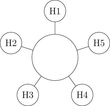
In this topology, each device is connected to two other devices on the network, forming a closed loop or a ring. Data is transmitted in one direction around the ring, from one device to another. This topology is simple and reliable, and it avoids collisions by using a token passing mechanism. However, it also has some limitations, such as low bandwidth, difficulty in adding or removing devices, and disruption of the network if one device fails or a cable breaks.

Like the bus organization, in a ring network, each host has a single physical interface connecting it to the ring. Any signal sent by a host on the ring will be received by all hosts attached to the ring. From a redundancy point of view, a single ring is not the best solution as the signal only travels in one direction on the ring; thus, if one of the links composing the ring is cut, the entire network fails. In practice, such rings have been used in local area networks, but are now often replaced by star-shaped networks. In metropolitan networks, rings are often used to interconnect multiple locations. In this case, two parallel links, composed of different cables, are often used for redundancy. With such a dual ring, when one ring fails all the traffic can be quickly switched to the other ring.

A network organized as a ring

Tree

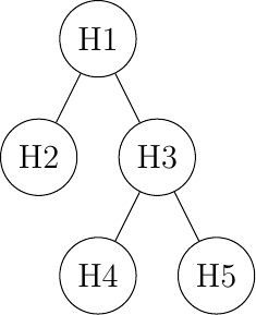
In this topology, multiple star networks are connected to each other by a bus network. The star networks act as branches of the tree and the bus network acts as the trunk of the tree. This topology combines the benefits of both star and bus topologies, such as scalability, flexibility, and ease of management. However, it also inherits some of their drawbacks, such as dependency on the central device and the bus cable. These networks are typically used when a large number of customers must be connected in a very cost-effective manner. Cable TV networks are often organized as trees.

A network organized as a tree

Full Mesh

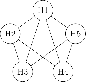
The full-mesh is the most reliable and highest performing network to interconnect these five hosts. However, this network organization has two important drawbacks. First, if a network contains N hosts, then N x (N -1) / 2 links are required. If the network contains more than a few hosts, it becomes impossible to lay down the required physical links. Second, if the network contains n hosts, then each host must have N-1 interfaces to terminate N-1 links, which is beyond the capabilities of most hosts. Furthermore, if a new host is added to the network, new links have to be laid down and one interface has to be added to each participating host. However, full-mesh has the advantage of providing the lowest delay between the hosts and the best resiliency against link failures. In practice, full-mesh networks are rarely used except when there are few network nodes and resiliency is key.

A full-mesh network

Hybrid

Hybrid topologies combine two or more basic topologies to form a more complex network configuration. For instance, a combination of star and bus topologies can be used to create a hybrid topology. Hybrid topologies are often used to achieve a balance between cost-effectiveness, scalability, and network resilience.

Watch this PowerCert overview of network topologies for an overview of network topologies (2018). [8:57]

Network Efficiency

In all these networks, except the full-mesh, the link bandwidth is shared among all connected hosts. Various algorithms have been proposed and are used to efficiently share the access to this resource. Some factors involved in these algorithms are discussed next.

Fairness

Sharing resources is important to ensure that the network efficiently serves its user. In practice, there are many ways to share resources. Some resource sharing schemes consider that some users are more important than others and should obtain more resources. For example, on the roads, police cars and ambulances have priority, or in some cities, traffic lanes are reserved for buses to promote public services.

In computer networks, the same problem of how to share resources arises. Given that resources are limited, the network needs to enable users to efficiently share them. Before designing an efficient resource sharing scheme, one needs to first formalize its objectives. In computer networks, the most popular objective for resource sharing schemes is that they must be fair. In a simple situation, for example two hosts using a shared 2 Mbps link, the sharing scheme should allocate the same bandwidth to each user, in this case 1 Mbps. However, in large networks, simply dividing the available resources by the number of users is not sufficient.

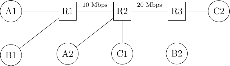
Consider the network shown in the figure below where A1 sends data to A2, B1 to B2, etc. In this network, how should we divide the bandwidth among the different flows? A first approach would be to allocate the same bandwidth to each flow. In this case, each flow would obtain 5 Mbps and the link between R2 and R3 would not be fully loaded (i.e., maximized). Another approach would be to allocate 10 Mbps to A1-A2, 20 Mbps to C1-C2 and nothing to B1-B2, as shown below. This is clearly unfair.

A small network

In large networks, fairness is always a compromise. The most widely used definition of fairness is the max-min fairness. A bandwidth allocation in a network is said to be max-min fair if it is such that it is impossible to allocate more bandwidth to one of the flows without reducing the bandwidth of a flow that already has a smaller allocation than the flow that we want to increase. If the network is completely known, it is possible to derive a max-min fair allocation as follows. Initially, all flows have a null bandwidth and they are placed in the candidate set. The bandwidth allocation of all flows in the candidate set is increased until one link becomes congested. At this point, the flows that use the congested link have reached their maximum allocation. They are removed from the candidate set and the process continues until the candidate set becomes empty.

In the above network, the allocation of all flows would grow until A1-A2 and B1-B2 reach 5 Mbps. At this point, link R1-R2 becomes congested and these two flows have reached their maximum. The allocation for flow C1-C2 can increase until reaching 15 Mbps. At this point, link R2-R3 is congested. To increase the bandwidth allocated to C1-C2, one would need to reduce the allocation to flow B1-B2. Similarly, the only way to increase the allocation to flow B1-B2 would require a decrease of the allocation to A1-A2.

Node Buffers

Network congestion is a situation where the demand for network resources exceeds the available capacity. This can cause delays, packet losses, and reduced network performance. One of the factors that can contribute to network congestion is the lack of node buffers.

Node buffers are memory spaces that store incoming or outgoing packets temporarily at each network node, such as a router or a switch. Node buffers help to smooth out the traffic fluctuations and to handle the mismatch between the input and output link speeds. Node buffers also enable some network protocols, such as TCP, to implement congestion control mechanisms that adjust the sending rate based on the feedback from the network.

However, node buffers are not unlimited and they can be exhausted when the traffic load is too high or too bursty. When there are not enough node buffers available, some packets have to be dropped or rejected by the network node. This can cause several problems:

Data loss: Some packets may contain important information that cannot be recovered or retransmitted easily, such as real-time audio or video streams. Losing these packets can degrade the quality of service and user experience.
Retransmission: Some packets may belong to reliable protocols, such as TCP, that require acknowledgment and retransmission of lost packets. Retransmitting these packets can increase the network load and congestion further, creating a vicious cycle.
Underutilization: Some packets may be dropped even when there is enough bandwidth available on the output link, because the node buffer is full. This can waste the network resources and reduce the network efficiency.

Therefore, it is important to design and manage node buffers properly to avoid or mitigate network congestion. Below are some possible solutions.

Buffer sizing: The size of node buffers should be optimized according to the network characteristics, such as link speed, round-trip time, traffic pattern, and congestion control algorithm. Buffers that are too small can cause frequent packet drops and underutilization, while buffers that are too large can cause excessive delays and buffer bloat.
Buffer management: The policy of how to allocate and deallocate node buffers should be fair and efficient. For example, some algorithms, such as random early detection (RED) or active queue management (AQM), can monitor the buffer occupancy and drop packets probabilistically before the buffer is full, to signal congestion and prevent buffer overflow.
Buffer sharing: The node buffers can be shared among different input or output ports, different traffic classes, or different flows, to improve the buffer utilization and flexibility. For example, some architectures, such as virtual output queueing (VOQ) or shared memory buffer (SMB), can dynamically allocate node buffers according to the traffic demand and priority.

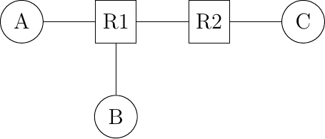
Sharing bandwidth among the hosts directly attached to a link is not the only sharing problem that occurs in computer networks. To understand the general problem, let us consider a very simple network which contains only point-to-point links. Besides the link bandwidth, the buffers on the network nodes are the second type of resource that needs to be shared inside the network. The node buffers play an important role in the operation of the network because that can be used to absorb transient traffic peaks. This network contains three hosts and two routers. All the links inside the network have the same capacity. For example, let us assume that all links have a bandwidth of 1000 bits per second and that the hosts send packets containing exactly one thousand bits.

A small network

Assume that on average host A and host B send a group of three packets every ten seconds. Their combined transmission rate (0.6 packets per second) is, on average, lower than the network capacity (1 packet per second). However, if they both start to transmit at the same time, node R1 will have to absorb a burst of packets. This burst of packets is a small network congestion.

This network congestion problem is one of the most difficult resource sharing problems in computer networks. Congestion occurs in almost all networks. Minimizing the amount of congestion is a key objective for many network operators. In most cases, they will have to accept transient congestion, i.e. congestion lasting a few seconds or perhaps minutes, but will want to prevent congestion that lasts days or months. For this, they can rely on a wide range of solutions. We briefly present some of these in the paragraphs below.

If R1 has enough buffers, it will be able to absorb the load without having to discard packets. The packets sent by hosts A and B will reach their final destination C, but will experience a longer delay than when they are transmitting alone. The amount of buffering on the network node is the first parameter that a network operator can tune to control congestion inside his network. Given the decreasing cost of memory, one could be tempted to put as many buffers as possible on the network nodes. Let us consider this case in the network above and assume that R1 has infinite buffers. Assume now that hosts A and B try to transmit a file that corresponds to one thousand packets each. Both are using a reliable protocol that relies on go-back-n to recover from transmission errors. The transmission starts and packets start to accumulate in R1’s buffers. The presence of these packets in the buffers increases the delay between the transmission of a packet by A and the return of the corresponding acknowledgment. Given the increasing delay, host A (and B as well) will consider that some of the packets that it sent have been lost. These packets will be retransmitted and will enter the buffers of R1. The occupancy of the buffers of R1 will continue to increase and the delays as well. This will cause new retransmissions. In the end, only one file will be delivered (very slowly) to the destination, but the link R1-R2 will transfer much more bytes than the size of the file due to the multiple copies of the same packets. This is known as the congestion collapse problem [RFC 896]. Congestion collapse is a nightmare for network operators. When it happens, the network carries packets without delivering useful data to the end users.

Congestion collapse is unfortunately not only an academic experience. Van Jacobson reports in [Jacobson1988] one of these events that affected him while he was working at the Lawrence Berkeley Laboratory (LBL). LBL was two network nodes away from the University of California in Berkeley. At that time, the link between the two sites had a bandwidth of 32 Kbps, but some hosts were already attached to 10 Mbps LANs. “In October 1986, the data throughput from LBL to UC Berkeley … dropped from 32 Kbps to 40 bps. We were fascinated by this sudden factor-of-thousand drop in bandwidth and embarked on an investigation of why things had gotten so bad.” This work lead to the development of various congestion control techniques that have allowed the Internet to continue to grow without experiencing widespread congestion collapse events.

Node Capacity

Besides bandwidth and memory, a third resource that needs to be shared inside a network is the packet processing capacity. To forward a packet, a router needs bandwidth on the outgoing link, but it also needs to analyze the packet header to perform a lookup inside its forwarding table. Performing these lookup operations require resources such as CPU cycles or memory accesses. Routers are usually designed to be able to sustain a given packet processing rate, measured in packets per second.

The performance of network nodes (either routers or switches) can be characterized by two key metrics :

The node’s capacity measured in bits per second

The node’s lookup performance measured in packets per second

The node’s capacity in bits per second mainly depends on the physical interfaces that it uses and also on the capacity of the internal interconnection (bus, crossbar switch, etc.) between the different interfaces inside the node. Many vendors, in particular for low-end devices, will use the sum of the bandwidth of the nodes’ interfaces as the node capacity in bits per second. Measurements do not always match this maximum theoretical capacity. A well designed network node will usually have a capacity in bits per second larger than the sum of its link capacities. Such nodes will usually reach this maximum capacity when forwarding large packets.

When a network node forwards small packets, its performance is usually limited by the number of lookup operations that it can perform every second. This lookup performance is measured in packets per second. The performance may depend on the length of the forwarded packets. The key performance factor is the number of minimal size packets that are forwarded by the node every second. This rate can lead to a capacity in bits per second, which is much lower than the sum of the bandwidth of the node’s links.

Let us now try to present a broad overview of the congestion problem in networks. We will assume that the network is composed of dedicated links having a fixed bandwidth. A network contains hosts that generate and receive packets and nodes (routers and switches) that forward packets. In practice, this largest demand is never reached and the network will be engineered to sustain a much lower traffic demand. The difference between the worst-case traffic demand and the sustainable traffic demand can be large, up to several orders of magnitude. Fortunately, the hosts can adapt their traffic demand to the current state of the network and the available bandwidth. For this, the hosts need to sense the current level of congestion and adjust their own traffic demand based on the estimated congestion. Network nodes can react in different ways to network congestion and hosts can sense the level of congestion in different ways.

Let us first explore which mechanisms can be used inside a network to control congestion and how these mechanisms can influence the behavior of the end hosts.

As explained earlier, one of the first manifestations of congestion on network nodes is the saturation of the network links that leads to a growth in the occupancy of the buffers of the node. This growth in buffer occupancy implies that some packets will spend more time in the buffer and thus in the network. If hosts measure the network delays (e.g. by measuring the round-trip-time between the transmission of a packet and the return of the corresponding acknowledgment), they could start to sense congestion. On low bandwidth links, a growth in the buffer occupancy can lead to an increase of the delays which can be easily measured by the end hosts. On high bandwidth links, a few packets inside the buffer will cause a small variation in the delay which may not necessarily be larger than the natural fluctuations of the delay measurements.

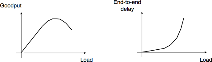
If the buffer’s occupancy continues to grow, it will overflow and packets will need to be discarded. Discarding packets during congestion is the second possible reaction of a network node to congestion. Before looking at how a node can discard packets, it is interesting to discuss the qualitative impact of the buffer occupancy on the reliable delivery of data through a network. This is illustrated by the figure below, adapted from [Jain1990].

../_images/jain.png — Network congestion

When the network load is low, buffer occupancy and link utilization are low. The buffers on the network nodes are mainly used to absorb very short bursts of packets, but on average the traffic demand is lower than the network capacity. If the demand increases, the average buffer occupancy will increase as well. Measurements have shown that the total throughput also increases. If the buffer occupancy is zero or very low, transmission opportunities on network links can be missed. This is not the case when the buffer occupancy is small but non zero. However, if the buffer occupancy continues to increase, the buffer becomes overloaded and the throughput does not increase anymore. When the buffer occupancy is close to the maximum, the throughput may decrease. This drop in throughput can be caused by excessive retransmissions of reliable protocols that incorrectly assume that previously sent packets have been lost while they are still waiting in the buffer. The network delay on the other hand increases with the buffer occupancy. In practice, a good operating point for a network buffer is a low occupancy to achieve high link utilization and also low delay for interactive applications.

Discarding packets is one of the signals that the network nodes can use to inform the hosts of the current level of congestion. Buffers on network nodes are usually used as FIFO queues to preserve packet ordering. Several packet discard mechanisms have been proposed for network nodes. These techniques basically answer two different questions :

What triggers a packet to be discarded? What are the conditions that lead a network node to decide to discard a packet? The simplest answer to this question is when the buffer is full. Although this is a good congestion indication, it is probably not the best one from a performance viewpoint. An alternative is to discard packets when the buffer occupancy grows too much. In this case, it is likely that the buffer will become full shortly. Since packet discarding is information that allows hosts to adapt their transmission rate, discarding packets early could allow hosts to react earlier and thus prevent congestion from happening.

Which packet(s) should be discarded? Once the network node has decided to discard packets, it needs to actually discard real packets.

By combining different answers to these questions, network researchers have developed different packet discard mechanisms.

Tail drop is the simplest packet discard technique. When a buffer is full, the arriving packet is discarded. Tail drop can be easily implemented. This is, by far, the most widely used packet discard mechanism. However, it suffers from two important drawbacks. First, since tail drop discards packets only when the buffer is full, buffers tend to be congested and real-time applications may suffer from increased delays. Second, tail drop is blind when it discards a packet. It may discard a packet from a low bandwidth interactive flow while most of the buffer is used by large file transfers.

Drop from front is an alternative packet discard technique. Instead of removing the arriving packet, it removes the packet that was at the head of the queue. Discarding this packet instead of the arriving one can have two advantages. First, it already stayed a long time in the buffer. Second, hosts should be able to detect the loss (and thus the congestion) earlier.

Probabilistic drop consists of various random drop techniques that have been proposed. A frequently cited technique is random early discard (RED) [FJ1993]. RED measures the average buffer occupancy and discards packets with a given probability when this average occupancy is too high. Compared to tail drop and drop from front, an advantage of RED is that thanks to the probabilistic drops, packets should be discarded from different flows in proportion of their bandwidth.

Discarding packets is a frequent reaction to network congestion. Unfortunately, discarding packets is not optimal since a packet which is discarded on a network node has already consumed resources on the upstream nodes. There are other ways for the network to inform the end hosts of the current congestion level. A first solution is to mark the packets when a node is congested. Several networking technologies have relied on this kind of packet marking.

In datagram networks, forward explicit congestion notification (FECN) can be used. One field of the packet header, typically one bit, is used to indicate congestion. When a host sends a packet, the congestion bit is unset. If the packet passes through a congested node, the congestion bit is set. The destination can then determine the current congestion level by measuring the fraction of the packets that it received with the congestion bit set. It may then return this information to the sending host to allow it to adapt its retransmission rate. Compared to packet discarding, the main advantage of FECN is that hosts can detect congestion explicitly without having to rely on packet losses.

In virtual circuit networks, packet marking can be improved if the return packets follow the reverse path of the forward packets. It this case, a network node can detect congestion on the forward path (e.g. due to the size of its buffer), but mark the packets on the return path. Marking the return packets (e.g. the acknowledgments used by reliable protocols) provides a faster feedback to the sending hosts compared to FECN. This technique is usually called backward explicit congestion notification (BECN).

If the packet header does not contain any bit in the header to represent the current congestion level, an alternative is to allow the network nodes to send a control packet to the source to indicate the current congestion level. Some networking technologies use such control packets to explicitly regulate the transmission rate of sources. However, their usage is mainly restricted to small networks. In large networks, network nodes usually avoid using such control packets. These control packets are even considered to be dangerous in some networks. First, using them increases the network load when the network is congested. Second, while network nodes are optimized to forward packets, they are usually pretty slow at creating new packets.

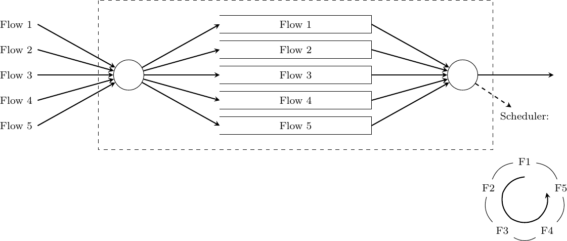
Dropping and marking packets is not the only possible reaction of a router that becomes congested. A router could also selectively delay packets belonging to some flows. There are different algorithms that can be used by a router to delay packets. If the objective of the router is to fairly distribute the bandwidth of an output link among competing flows, one possibility is to organize the buffers of the router as a set of queues. For simplicity, let us assume that the router is capable of supporting a fixed number of concurrent flows, say N. One queue of the router is associated to each flow and when a packet arrives, it is placed at the tail of the corresponding queue. All the queues are controlled by a scheduler. A scheduler is an algorithm that is run each time there is an opportunity to transmit a packet on the outgoing link. Various schedulers have been proposed in the scientific literature and some are used in real routers.

A very simple scheduler is the round-robin scheduler. This scheduler serves all the queues in a round-robin fashion. If all flows send packets of the same size, then the round-robin scheduler fairly allocates the bandwidth among the different flows. Otherwise, it favors flows that are using larger packets.

A round-robin scheduler, where N = 5

Load Distribution

Delays, packet discards, packet markings and control packets are the main types of information that the network can exchange with the end hosts. Discarding packets is the main action that a network node can perform if the congestion is too severe. Besides tackling congestion at each node, it is also possible to divert some traffic flows from heavily loaded links to reduce congestion.

Early routing algorithms [MRR1980] have used delay measurements to detect congestion between network nodes and update the link weights dynamically. By reflecting the delay perceived by applications in the link weights used for the shortest paths computation, these routing algorithms managed to dynamically change the forwarding paths in reaction to congestion. However, deployment experience showed that these dynamic routing algorithms could cause oscillations and did not necessarily lower congestion.

Deployed datagram networks rarely use dynamic routing algorithms, except in some wireless networks. In datagram networks, the state of the art reaction to long term congestion, i.e., congestion lasting hours, days or more, is to measure the traffic demand and then select the link weights [FRT2002] that allow minimizing the maximum link loads. If the congestion lasts longer, changing the weights is not sufficient anymore and the network needs to be upgraded with additional or faster links. However, in wide area networks, adding new links can take months. In virtual circuit networks, another way to manage or prevent congestion is to limit the number of circuits that use the network at any time. This technique is usually called connection admission control. When a host requests the creation of a new circuit in the network, it specifies the destination and in some networking technologies the required bandwidth. With this information, the network can check whether there are enough resources available to reach this particular destination. If yes, the circuit is established. If not, the request is denied and the host will have to defer the creation of its virtual circuit. Connection admission control schemes are widely used in the telephone networks. In these networks, a busy tone corresponds to an unavailable destination or a congested network. In datagram networks, this technique cannot be easily used since the basic assumption of such a network is that a host can send any packet towards any destination at any time. A host does not need to request the authorization of the network to send packets towards a particular destination.

Based on the feedback received from the network, the hosts can adjust their transmission rate. Another way to share the network resources is to distribute the load across multiple links. Many techniques have been designed to spread the load over the network. As an illustration, let us briefly consider how the load can be shared when accessing some content. Consider a large and popular file such as the image of a Linux distribution or the upgrade of a commercial operating system that will be downloaded by many users. There are many ways to distribute this large file. A naive solution is to place one copy of the file on a server and allow all users to download this file from the server. If the file is popular and millions of users want to download it, the server will quickly become overloaded.

There are two classes of solutions that can be used to serve a large number of users.

A first approach is to store the file on servers whose name is known by the clients. Before retrieving the file, each client will query the name service to obtain the address of the server. If the file is available from many servers, the name service can provide different addresses to different clients. This will automatically spread the load since different clients will download the file from different servers. Most large content providers use such a solution to distribute large files or videos.
Another solution allows spreading the load among many sources without relying on the name service. To retrieve a file, a client needs to retrieve all the blocks that compose the file. However, nothing forces the client to retrieve all the blocks in sequence and from the same server. Each file is associated with metadata that indicates for each block a list of addresses of hosts that store this block. To retrieve a complete file, a client first downloads the metadata. Then, it tries to retrieve each block from one of the hosts that store the block. In practice, implementations often try to download several blocks in parallel. Once one block has been successfully downloaded, the next block can be requested. If a host is slow to provide one block or becomes unavailable, the client can contact another host listed in the metadata. Content providers can allow the clients to participate in the distribution of blocks. Once a client has downloaded one block, it contacts the server which stores the metadata to indicate that it can also provide this block. With this scheme, when a file is popular, its blocks are downloaded by many hosts that automatically participate in the distribution of the blocks. Thus, the number of servers that are capable of providing blocks from a popular file automatically increases with the file’s popularity.

Collisions

Now that we have provided a broad overview of the techniques that can be used to spread the load and allocate resources in the network, let us analyze two techniques in more detail: medium access control and congestion control.

Medium Access Control (MAC) Algorithms

The common problem among LANs is how to efficiently share the available bandwidth. If two devices send a frame at the same time, the two electrical, optical or radio signals that correspond to these frames will appear at the same time on the transmission medium and a receiver will not be able to decode either frame. Such simultaneous transmissions are called collisions. A collision may involve frames transmitted by two or more devices attached to the LAN. Collisions are the main cause of errors in wired LANs.

All LAN technologies rely on a medium access control algorithm to regulate the transmissions to either minimize or avoid collisions. There are two broad families of medium access control algorithms :

Deterministic or pessimistic MAC algorithms assume that collisions are a very severe problem and that they must be completely avoided. These algorithms ensure that at any time, at most one device is allowed to send a frame on the LAN. This is usually achieved by using a distributed protocol that elects one device that is allowed to transmit at each time. A deterministic MAC algorithm ensures that no collision will happen, but there is some overhead in regulating the transmission of all the devices attached to the LAN. Examples include FDMA, TDMA, and Token Ring.

Stochastic or optimistic MAC algorithms assume that collisions are part of the normal operation of a LAN. They aim to minimize the number of collisions, but they do not try to avoid all collisions. Stochastic algorithms are usually easier to implement than deterministic ones. Stochastic or optimistic MAC algorithms assume that collisions are not a very severe problem and that they can be tolerated or resolved. These algorithms allow multiple devices to send frames on the LAN at the same time, without requiring a strict coordination or reservation mechanism. A stochastic MAC algorithm may cause some collisions, but it also reduces the overhead and increases the network throughout. Examples include CSMA/CA and CSMA/CD.

Certainly, medium access control (MAC) mechanisms play a crucial role in regulating the access to shared communication channels in network environments. These mechanisms are essential for managing the allocation of available bandwidth and ensuring efficient data transmission. Below is a summary of some common medium access control mechanisms.

Static Allocation Methods

A first solution to share the available resources among all the devices attached to one LAN is to define, a priori, the distribution of the transmission resources among the different devices. Static allocation schemes for media access control algorithms are methods of dividing the capacity of a shared communication channel among multiple users or devices by using fixed portions. Each user or device is assigned a portion of the channel for all time, regardless of whether it has data to transmit or not. If the user or device has no data to transmit, its portion goes unused. Static allocation schemes can use various techniques, such as frequency division multiplexing (FDM), time division multiplexing (TDM), or code division multiplexing (CDM), to split the channel into frequency bands, time slots, or codes, respectively. Below are some of the major static allocation schemes.

Frequency Division Multiple Access (FDMA): In this scheme, each user or device is assigned a fixed frequency band in which it can transmit data. The frequency bands are non-overlapping and cover the entire spectrum of the transmission channel. These scheme avoids collisions by dividing the channel into non-overlapping frequency ranges, but it also limits the number of users or devices that can be supported by the available spectrum.
Time Division Multiple Access (TDMA): In this scheme, each user or device is assigned a fixed time slot in which it can transmit data. The time slots are repeated in a cycle, and each user or device knows its own slot and the slots of other users or devices. This scheme avoids collisions by dividing the channel into non-overlapping time intervals, but it also wastes bandwidth if some users or devices have nothing to transmit in their slots.
Code Division Multiple Access (CDMA): CDMA can be seen as a static allocation scheme, because each user is assigned a code for all time, regardless of whether it has data to transmit or not. The code acts as a fixed portion of the channel that belongs to the user. In this scheme, each user or device is assigned a unique code that modulates its data signal. The codes are orthogonal to each other, which means they have zero correlation. The signals from different users or devices are transmitted simultaneously over the same channel, and they are separated at the receiver by using the corresponding codes. These scheme avoids collisions by using codes that are independent of each other, but it also required complex encoding and decoding techniques.

Dynamic Allocation Methods

Using a static allocation scheme for computers attached to a LAN would lead to huge inefficiencies, despite the fact that the other computers are in their off period and thus do not need to transmit any information. The dynamic MAC algorithms discussed next aim to solve this problem.

Dynamic allocation schemes for media access controls are methods of dividing the capacity of a shared communication channel among multiple users or devices by using variable portions. Each user or device is assigned a portion of the channel only when it has data to transmit, and releases it when it is done. This way, dynamic allocation schemes can adapt to the changing traffic patterns and demands of the users or devices, and improve the efficiency and utilization of the channel. Dynamic allocation schemes can use different techniques, such as random access, reservation, or polling, to coordinate the access of multiple users of devices to the channel.

Some examples of dynamic allocation schemes are described below:

Random access: In this scheme, each user or device can transmit data whenever it wants, without any prior coordination or reservation. However, this also means that there is a possibility of collisions, which occur when two or more users or devices try to transmit data at the same time and interfere with each other. To deal with collisions, random access schemes use different mechanisms, such as collision detection, collision avoidance, or retransmission. Some examples of random access schemes are ALOHA, CSMA, and CSMA/CA.
Reservation: In this scheme, each user or device has to reserve a portion of the channel before transmitting data. The reservation can be done by using a separate control channel, or by using special control frames on the data channel. The reservation can be either fixed or variable in duration, depending on the amount of data to be transmitted. Reservation schemes can avoid collisions by granting exclusive access to the channel to one user or device at a time. Some examples of reservation schemes are TDMA, FDMA, and CDMA. Note that CDMA can also be seen as a dynamic allocation scheme, because the number of users that can be supported by the channel is not fixed, but depends on the interference level and the quality requirement. The channel can accommodate more users by reducing the quality or increasing the interference tolerance.
Polling: In this scheme, there is a central controller that polls each user or device periodically and asks if it has any data to transmit. If the user or device has data to transmit, it sends it to the controller or directly to the destination. If not, it waits for the next poll. Polling schemes can avoid collisions by regulating the access of multiple users or devices to the channel according to a predefined order. Some examples of polling schemes are token ring, token bus, and wireless USB.

ALOHA and CSMA are two types of random access protocols that are used to control the access of multiple devices to a shared communication channel. ALOHA was the first random access protocol that was developed for wireless networks, while CSMA was an improvement over ALOHA that was adopted by wired networks such as Ethernet.

ALOHA was designed in 1971 by Norman Abramson and his colleagues at the University of Hawaii. The basic idea of ALOHA was that any device could transmit data whenever it had something to send, without sensing the channel or waiting for an acknowledgment. However, this also meant that collisions could occur frequently, as two or more devices could transmit data at the same time and interfere with each other. To deal with collisions, ALOHA used a simple retransmission scheme. If a device did not receive an acknowledgment within a certain time, it assumed that a collision had occurred and retransmitted the data after a random delay. In this algorithm, each device sends data whenever it has something to transmit, without listening to the medium or waiting for an acknowledgment. The receiver sends an acknowledgment for each correctly received frame. If the sender does not receive an acknowledgment within a certain time, it assumes that a collision has occurred and retransmits the frame. ALOHA is simple and robust, but has a low efficiency and a high collision probability. ALOHA and slotted ALOHA can easily be implemented, but unfortunately, they can only be used in networks that are very lightly loaded. Designing a network for a very low utilization is possible, but it clearly increases the cost of the network. To overcome the problems of ALOHA, many MAC mechanisms have been proposed to improve channel utilization.

Carrier Sense Multiple Access

CSMA stands for Carrier Sense Multiple Access, and it was developed in the late 1970s by Robert Metcalfe and David Boggs at Xerox PARC. The main idea of CSMA was that before transmitting data, a device would sense the channel and check if it was idle or busy. If the channel was idle, the device would transmit data immediately; if the channel was busy, the device would defer its transmission before attempting to transmit again. This way, CSMA could reduce the probability of collisions by avoiding simultaneous transmissions. However, CSMA could not eliminate collisions completely, as two or more devices could still sense the channel as idle at the same time and start transmitting data. To handle collisions, CSMA used different techniques, such as collision detection (CSMA/CD) or collision avoidance (CSMA/CA).

CSMA was an improvement over ALOHA in terms of network performance and efficiency, as it could achieve higher throughput and lower delay by reducing collisions. CSMA also had more flexibility and scalability than ALOHA, as it could adapt to different network conditions and traffic patterns by adjusting the sensing and backoff parameters. CSMA became the dominant random access protocol for wired networks such as Ethernet, while ALOHA remained popular for wireless networks such as satellite communications.

Carrier Sense Multiple Access (CSMA) is a significant improvement compared to ALOHA. CSMA requires all nodes to listen to the transmission channel to verify that it is free before transmitting a frame [KT1975]. When a node senses the channel to be busy, it defers its transmission until the channel becomes free again. The pseudocode below provides a more detailed description of the operation of CSMA.

# persistent CSMA
N = 1
while N <= max:
    wait(channel_becomes_free)
    send(frame)
    wait(ack or timeout)
    if ack:
       break  # transmission was successful
    else:
       # timeout
       N = N + 1
else:
    # too many transmission attempts

The above pseudocode is often called persistent CSMA [KT1975] as the terminal will continuously listen to the channel and transmit its frame as soon as the channel becomes free. Another important variant of CSMA is the non-persistent CSMA [KT1975]. The main difference between persistent and non-persistent CSMA described in the pseudocode below is that a non-persistent CSMA node does not continuously listen to the channel to determine when it becomes free. When a non-persistent CSMA terminal senses the transmission channel to be busy, it waits for a random time before sensing the channel again. This improves channel utilization compared to persistent CSMA. With persistent CSMA, when two terminals sense the channel to be busy, they will both transmit (and thus cause a collision) as soon as the channel becomes free. With non-persistent CSMA, this synchronization does not occur, as the terminals wait a random time after having sensed the transmission channel. However, the higher channel utilization achieved by non-persistent CSMA comes at the expense of a slightly higher waiting time in the terminals when the network is lightly loaded.

# Non persistent CSMA
N = 1
while N <= max:
    listen(channel)
    if free(channel):
        send(frame)
        wait(ack or timeout)
        if received(ack):
           break  # transmission was successful
        else:
           # timeout
           N = N + 1
    else:
        wait(random_time)
else:
    # too many transmission attempts

[KT1975] analyzes in detail the performance of several CSMA variants. Under some assumptions about the transmission channel and the traffic, the analysis compares ALOHA, slotted ALOHA, persistent and non-persistent CSMA. Under these assumptions, ALOHA achieves a channel utilization of only 18.4% of the channel capacity. Slotted ALOHA is able to use 36.6% of this capacity. Persistent CSMA improves the utilization by reaching 52.9% of the capacity while non-persistent CSMA achieves 81.5% of the channel capacity.

Carrier Sense Multiple Access with Collision Detection

CSMA/CD (Carrier Sense Multiple Access with Collision Detection): CSMA/CD is an enhancement of the CSMA protocol, primarily used in Ethernet networks. In this mechanism, if a collision is detected during data transmission, the devices involved stop transmitting, wait for a random amount of time, and then reattempt transmission.

CSMA improves channel utilization compared to ALOHA. However, the performance can still be improved, especially in wired networks. Consider the situation of two terminals that are connected to the same cable. This cable could, for example, be a coaxial cable as in the early days of Ethernet [Metcalfe1976]. It could also be built with twisted pairs.

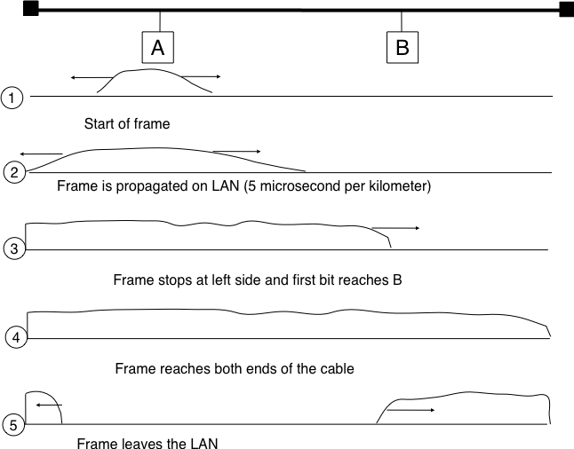
Before extending CSMA, it is useful to understand, more intuitively, how frames are transmitted in such a network and how collisions can occur. The figure below illustrates the physical transmission of a frame on such a cable. To transmit its frame, host A must send an electrical signal on the shared medium. The first step is thus to begin the transmission of the electrical signal. This is point (1) in the figure below. This electrical signal will travel along the cable. Although electrical signals travel fast, we know that information cannot travel faster than the speed of light (i.e. 300.000 kilometers/second). On a coaxial cable, an electrical signal is slightly slower than the speed of light and 200.000 kilometers per second is a reasonable estimation. This implies that if the cable has a length of one kilometer, the electrical signal will need 5 microseconds to travel from one end of the cable to the other. The ends of coaxial cables are equipped with termination points that ensure that the electrical signal is not reflected back to its source. This is illustrated at point (3) in the figure, where the electrical signal has reached the left endpoint and host B. At this point, B starts to receive the frame being transmitted by A. Notice that there is a delay between the transmission of a bit on host A and its reception by host B. If there were other hosts attached to the cable, they would receive the first bit of the frame at slightly different times. As we will see later, this timing difference is a key problem for MAC algorithms. At point (4), the electrical signal has reached both ends of the cable and occupies it completely. Host A continues to transmit the electrical signal until the end of the frame. As shown at point (5), when the sending host stops its transmission, the electrical signal corresponding to the end of the frame leaves the coaxial cable. The channel becomes empty again once the entire electrical signal has been removed from the cable.

../_images/frame-bus.png — Frame transmission on a shared bus

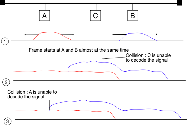
Now that we have looked at how a frame is actually transmitted as an electrical signal on a shared bus, it is interesting to look in more detail at what happens when two hosts transmit a frame at almost the same time. This is illustrated in the figure below, where hosts A and B start their transmission at the same time (point (1)). At this time, if host C senses the channel, it will consider it to be free. This will not last a long time and at point (2) the electrical signals from both host A and host B reach host C. The combined electrical signal (shown graphically as the superposition of the two curves in the figure) cannot be decoded by host C. Host C detects a collision, as it receives a signal that it cannot decode. Since host C cannot decode the frames, it cannot determine which hosts are sending the colliding frames. Note that host A (and host B) will detect the collision after host C (point (3) in the figure below).

../_images/frame-collision.png — Frame collision on a shared bus

As shown above, hosts detect collisions when they receive an electrical signal that they cannot decode. In a wired network, a host is able to detect such a collision both while it is listening (e.g., like host C in the figure above) and also while it is sending its own frame. When a host transmits a frame, it can compare the electrical signal that it transmits with the electrical signal that it senses on the wire. At points (1) and (2) in the figure above, host A senses only its own signal. At point (3), it senses an electrical signal that differs from its own signal and can thus detects the collision. At this point, its frame is corrupted and it can stop its transmission.

The ability to detect collisions while transmitting is the starting point for the Carrier Sense Multiple Access with Collision Detection (CSMA/CD) MAC algorithm, which is used in Ethernet networks [Metcalfe1976] [IEEE802.3] . When an Ethernet host detects a collision while it is transmitting, it immediately stops its transmission. Compared with pure CSMA, CSMA/CD is an important improvement since when collisions occur, they only last until colliding hosts have detected it and stopped their transmission. In practice, when a host detects a collision, it sends a special jamming signal on the cable to ensure that all hosts have detected the collision.

Furthermore, on the wired networks where CSMA/CD is used, collisions are almost the only cause of transmission errors that affect frames. Transmission errors that only affect a few bits inside a frame seldom occur in these wired networks. For this reason, the designers of CSMA/CD chose to completely remove the acknowledgment frames in the data link layer. When a host transmits a frame, it verifies whether its transmission has been affected by a collision. If not, given the negligible bit error ratio of the underlying network, it assumes that the frame was received correctly by its destination. Otherwise the frame is retransmitted after some delay.

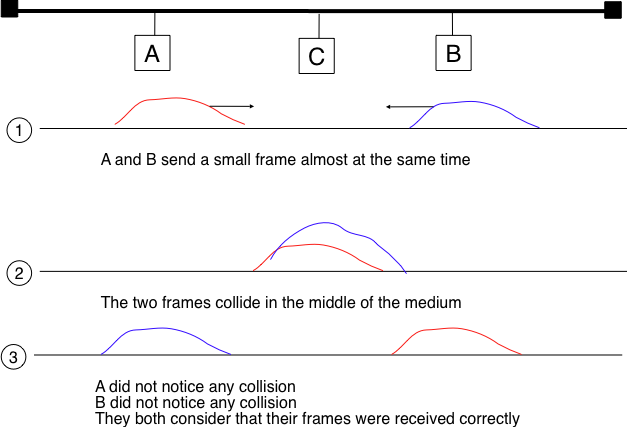
Removing acknowledgments is an interesting optimization as it reduces the number of frames that are exchanged on the network and the number of frames that need to be processed by the hosts. However, to use this optimization, we must ensure that all hosts will be able to detect all the collisions that affect their frames. The problem is important for short frames. Let us consider two hosts, A and B, that are sending a small frame to host C as illustrated in the figure below. If the frames sent by A and B are very short, the situation illustrated below may occur. Hosts A and B send their frame and stop transmitting (point (1)). When the two short frames arrive at the location of host C, they collide and host C cannot decode them (point (2)). The two frames are absorbed by the ends of the wire. Neither host A nor host B have detected the collision. They both consider their frame to have been received correctly by its destination.

../_images/frame-collision-short.png — The short-frame collision problem

However, collision detection is not perfect because of the short-frame collision problem. This problem occurs when a device sends a short frame (a data packet that is smaller than the maximum allowed size) and another device starts sending a frame after the first device has finished, but before the first frame has reached the other end of the medium. In this case, the first device will not detect the collision, because it has already stopped monitoring the medium, but the second device will detect the collision and stop sending. This will result in data loss and wasted bandwidth.

To solve the short-frame collision problem, CSMA/CD uses a concept called slot time. Slot time is the minimum time that a device must wait before sending a frame after sensing that the medium is idle. Slot time is also the minimum time that a device must monitor the medium while sending a frame. Slot time is calculated based on the propagation delay of the medium, which is the maximum time it takes for a signal to travel from one end of the medium to the other. Slot time ensures that if a collision occurs, it will be detected by both devices involved in the collision, regardless of the frame size.

For example, suppose that the propagation delay of the medium is 15 microseconds, and the slot time is 30 microseconds (twice the propagation delay). If device A sends a short frame of 10 microseconds, and device B starts sending a frame after 5 microseconds, there will be a collision at 20 microseconds. Device A will detect the collision at 35 microseconds (20 + 15), and device B will detect the collision at 25 microseconds (10 + 15). Both devices will stop sending and wait for a random time before trying again.

The complete pseudo-code for the CSMA/CD algorithm is shown in the figure below.

# CSMA/CD pseudo-code
N = 1
while N <= max:
    wait(channel_becomes_free)
    send(frame)
    wait_until (end_of_frame) or (collision)
    if collision detected:
        stop_transmitting()
        send(jamming)
        k = min(10, N)
        r = random(0, 2**k - 1)
        wait(r * slotTime)
        N = N + 1
    else:
        wait(inter-frame_delay)
        break  # transmission was successful
else:
    # too many transmission attempts

The inter-frame delay used in this pseudo-code is a short delay corresponding to the time required by a network adapter to switch from transmit to receive mode. It is also used to prevent a host from sending a continuous stream of frames without leaving any transmission opportunities for other hosts on the network. This contributes to the fairness of CSMA/CD. Despite this delay, there are still conditions where CSMA/CD is not completely fair [RY1994]. Consider for example a network with two hosts : a server sending long frames and a client sending acknowledgments. Measurements reported in [RY1994] have shown that there are situations where the client could suffer from repeated collisions that lead it to wait for long periods of time due to the exponential back-off algorithm.

Carrier Sense Multiple Access with Collision Avoidance

CSMA/CA (Carrier Sense Multiple Access with Collision Avoidance) is used in wireless networks to avoid collisions that may occur due to hidden node problems. The Carrier Sense Multiple Access with Collision Avoidance (CSMA/CA) Medium Access Control algorithm was designed for the popular WiFi wireless network technology [IEEE802.11]. CSMA/CA also senses the transmission channel before transmitting a frame. Furthermore, CSMA/CA tries to avoid collisions by carefully tuning the timers used by CSMA/CA devices.

The basic idea behind CSMA/CA is the “Listen Before Talk” (LBT) principle, which means that a device checks the channel before sending data, and waits for a certain time if the channel is busy. However, this is not enough to avoid collisions completely, as two or more devices may still start sending data at the same time. To deal with this problem, CSMA/CA relies on a backoff timer.

The backoff timer works as follows:

Before sending data, a device senses the channel and checks if it is idle or busy. If the channel is idle, the device starts transmitting data immediately. If the channel is busy, the device waits for a random time before trying again.
The random time is chosen from a range of values that depends on the number of attempts that the device has made to send data. The range of values increases exponentially with each attempt, to reduce the likelihood of another collision occurring. For example, if the device has made one attempt, it chooses a random time from 0 to 1 slot time; if it has made two attempts, it chooses a random time from 0 to 3 slot times; and so on.
The slot time is the minimum time that a device must wait before sending data after sensing that the medium is idle. The slot time is calculated based on the propagation delay of the medium, which is the maximum time it takes for a signal to travel from one end of the medium to the other.
The device counts down the backoff timer while sensing the channel. If the channel becomes busy during the countdown, the device freezes the backoff timer and resumes it when the channel becomes idle again. If the channel remains idle until the backoff timer reaches zero, the device transmits data.

The backoff timer helps to avoid or resolve collisions by making devices wait different periods of time and avoiding simultaneous transmissions. The backoff timer also improves the network performance and efficiency by reducing the number of retransmissions and wasted bandwidth.

The pseudo-code below summarizes the operation of a CSMA/CA device. The values of the SIFS (short interframe space), DIFS (distributed interframe space), and EIFS (extended interframe space) depend on the underlying physical layer technology [IEEE802.11]

# CSMA/CA simplified pseudo-code
N=1
while N <= max:
    wait_until(free(channel))
    if correct(last_frame):
        wait(channel_free_during_t >= DIFS)
    else:
        wait(channel_free_during_t >= EIFS)

    backoff_time = int(random(0, min(255, 7 * ( 2 ** (N - 1))))) * slot_time
    wait(channel free during backoff_time)
    # backoff timer is frozen while channel is sensed to be busy
    send(frame)
    wait(ack or timeout)
    if received(ack)
        # frame received correctly
        break
    else:
        # retransmission required
        N = N + 1
else:
    # too many transmission attempts

Another problem faced by wireless networks is often called the hidden station problem. In a wireless network, radio signals are not always propagated same way in all directions. For example, two devices separated by a wall may not be able to receive each other’s signal while they could both be receiving the signal produced by a third host. This is illustrated in the figure below, but it can happen in other environments. For example, two devices that are on different sides of a hill may not be able to receive each other’s signal while they are both able to receive the signal sent by a station at the top of the hill. Furthermore, the radio propagation conditions may change with time. For example, a truck may temporarily block the communication between two nearby devices.

../_images/csmaca-hidden.svg — The hidden station problem

To avoid collisions in these situations, CSMA/CA allows devices to reserve the transmission channel for some time. This is done by using the two control frames: Request To Send (RTS) and Clear To Send (CTS). Both are very short frames to minimize the risk of collisions. To reserve the transmission channel, a device sends a RTS frame to the intended recipient of the data frame. The RTS frame contains the duration of the requested reservation. The recipient replies, after a SIFS delay, with a CTS frame which also contains the duration of the reservation. As the duration of the reservation has been sent in both RTS and CTS, all hosts that could collide with either the sender or the reception of the data frame are informed of the reservation. They can compute the total duration of the transmission and defer their access to the transmission channel until then.

The utilization of the reservations with CSMA/CA is an optimization that is useful when collisions are frequent. If there are few collisions, the time required to transmit the RTS and CTS frames can become significant and in particular when short frames are exchanged. Some devices only turn on RTS/CTS after transmission errors.

Watch PowerCert’s explanation of CSMA-CD and CSMA-CA (2019). [6:13]

Deterministic Medium Access Control Algorithms

Deterministic methods of medium access control (MAC) are protocols that ensure that only one device can transmit data on a shared communication channel at a time, and that the transmission delay is predictable and bounded. Deterministic MAC protocols are suitable for applications that require real-time communication and reliability, such as industrial automation, voice over IP, or multimedia streaming.

Historically, deterministic MAC protocols were proposed and standardized in the 1970s and 1980s by different factions of the networking community, who disagreed on the best way to fulfill the needs of local area networks (LANs). The IEEE 802 committee created three working groups to develop three different LAN technologies based on deterministic MAC protocols: IEEE 802.3 for CSMA/CD, IEEE 802.4 for Token Bus, and IEEE 802.5 for Token Ring. These protocols used different techniques, such as tokens, reservations, or polling, to coordinate the access of multiple devices to the channel.

However, deterministic MAC protocols also had some drawbacks, such as complexity, cost, scalability, and waste of resources. They were gradually replaced by more efficient and flexible protocols, such as Ethernet, which used optimistic MAC protocols based on random access and collision resolution. Ethernet became the dominant LAN technology by the 1990s and deterministic MAC protocols became obsolete or niche.

Currently, deterministic MAC protocols are still relevant for some applications and domains that require high performance and quality of service. For example, some wireless networks use deterministic MAC protocols to avoid or minimize collisions and interference in the shared wireless medium. Some examples of wireless networks that use deterministic MAC protocols are WirelessHART, ISA100.11a, or IEEE 802.15.4e. These protocols use techniques such as time division multiple access (TDMA), frequency division multiple access (FDMA), or code division multiple access (CDMA), to divide the channel into non-overlapping portions for different devices.

Congestion Control

Most networks contain links having different bandwidth. Some hosts can use low bandwidth wireless networks. Some servers are attached via 10 Gbps interfaces and inter-router links may vary from a few tens of kilobits per second up to hundred Gbps. Despite these huge differences in performance, any host should be able to efficiently exchange segments with a high-end server.

Congestion control aims to prevent or reduce the negative effects of network congestion, which is a situation where the demand for network resources exceeds the available capacity. Network congestion can cause delays, packet losses, and reduced network performance. Congestion control can be implemented at different layers of the network stack, such as the data link layer, the network later, or the transport later.

Some congestion control schemes rely on a close cooperation between the end hosts and the routers, while others are mainly implemented on the end hosts with limited support from the routers.

Congestion collapse is a phenomenon that occurs when the network becomes overloaded with too many packets, resulting in high delays, low throughput, and high packet losses. Congestion collapse can severely degrade the network performance and efficiency, and even render it unusable, particularly when stochastic MAC algorithms are used in networks with high traffic load and low channel capacity. In such networks, collisions become frequent and retransmissions consume a large portion of the channel bandwidth. This leads to a vicious cycle, where more packets are injected into the network than the network can handle, resulting in more collisions, more retransmissions, and more congestion. Congestion collapse can be avoided by using different techniques. [Jacobson1988]

Backoff algorithms: These are mechanisms that make devices wait for a random time before attempting to transmit data again after a collision. The random time is chosen from a range of values that increases exponentially with each collision. This reduces the probability of repeated collisions and spreads out the traffic load over time.
Window policy: This is a mechanism that limits the number of packets that a device can send or receive at a time. The window size is adjusted dynamically based on the network conditions, such as the number of acknowledgments received or the number of packets lost. This regulates the sending rate and prevents the device from overwhelming the channel or the receiver.
Discarding policy: This is a mechanism that drops or rejects packets when the channel or the buffer is full. The discarding policy can be based on different criteria, such as packet priority, packet age, or packet source. This prevents buffer overflow and reduces congestion.
Acknowledgment policy: This is a mechanism that sends feedback from the receiver to the sender about the status of the packets received. The feedback can be positive (acknowledgment) or negative (negative acknowledgment or request for retransmission). The feedback can also include information about the channel condition, such as congestion indication or available window size. This helps the sender to adjust its sending rate and retransmit only the lost packets.
Admission policy: This is a mechanism that controls the entry of new packets into the network based on the availability of network resources, such as bandwidth or buffer space. The admission policy can be based on different criteria, such as packet type, packet source, or packet destination. This prevents congestion before it happens and maintains quality of service.

One of the emerging trends with congestion control in networks is the use of binary feedback, which is a simple and efficient way of sending information from the network to the users about the congestion level. Binary feedback can be either explicit or implicit. Explicit binary feedback means that the network explicitly signals congestion to the users by setting a bit on the packets or sending special control messages. Implicit binary feedback means that the users infer congestion from the network behavior, such as packet losses or delays. Binary feedback can help users adjust their sending rate and avoid or resolve congestion.

Some examples of congestion control algorithms that use binary feedback as as follows:

Binary Increase Congestion Control (BIC): This is a TCP congestion control algorithm that uses a binary search algorithm to find the optimal window size. BIC uses implicit binary feedback from packet losses to detect congestion and adjust its window size accordingly. BIC is designed for fast log-distance networks, where it can achieve high throughout and stability.
A Binary Feedback Scheme for Congestion Avoidance in Computer Networks: This is a MAC algorithm that uses explicit binary feedback from routers to regulate the access of multiple users to a shared channel. The routers set a congestion-indication bit on packets flowing in the forward direction, and the users adjust their sending rate based on the feedback received from the acknowledgments. This scheme is distributed, adaptive, and fair.
Effective IoT Congestion Control Using Binary Feedback: This is a MAC algorithm that uses explicit binary feedback from gateways to control the access of multiple IoT devices to a shared wireless channel. The gateways send a busy tone signal to indicate congestion to the IoT devices, and the devices use a backoff algorithm to defer their transmissions until the channel is free. This scheme is simple, robust, and scalable.

Learn more about the history of congestion control from ComputerPhile’s Dr. Richard Clegg (2022). [20:15]

Virtual LANs (VLANs)

In contemporary networking, virtual LANs (VLANs) play a pivotal role in network design, management, and security. VLANs are a logical network concept that enables the segmentation of a single physical network into multiple virtual networks, each functioning as an independent entity. Unlike traditional LANs, which rely solely on physical infrastructure for network segmentation, VLANs operate at the data link layer (Layer 2) of the OSI model, facilitating the creation of distinct broadcast domains within a shared physical network. This section provides an overview of VLANs, their advantages, implementation, and a comparison with traditional LANs.

Virtual LANs (VLANs) are a means to partition a network into isolated segments that can be managed independently. Unlike traditional LANs, which depend on physical separation of devices, VLANs provide logical separation. VLANs achieve this by tagging Ethernet frames with a VLAN identifier, which indicates to network switches how to treat the traffic. Devices within the same VLAN can communicate as if they are on the same physical network, even if they are physically dispersed. VLANs can be organized by criteria such department, function, or security requirements, and they allow network administrators to better control broadcast domains and optimize network traffic.

While LANs can span across multiple switches, they are fundamentally bounded by the physical infrastructure. VLANs, on the other hand, transcend physical boundaries, making them more flexible and scalable for complex network architectures. Moreover, VLANs allow for the creation of multiple broadcast domains within a single physical network, enhancing security and network management by isolating traffic and access based on criteria such as function or security requirements. A virtual local area network (VLAN) can appear to be on the same LAN irrespective of the physical configuration of the underlying network. VLANs are created by applying tags to network frames and handling these tags in networking devices, such as switches and routers.

A VLAN typically uses multiple broadcast domains, which means that devices on different VLANs cannot communicate with each other directly without requiring a router. A VLAN can use different techniques, such as frequency division multiplexing (FDM), time division multiplexing (TDM), or code division multiplexing (CDM), to split the network into frequency bands, time slots, or codes, respectively.

Essentially, VLANs can improve the performance, security, and management of LANs of a single physical network by creating the appearance and functionality of separate networks.

VLANs can increase network performance by reducing broadcast traffic and congestion. Creating logical sub-networks limits broadcast traffic in workgroups or to a defined set of users.
VLANs can enhance network security by isolating devices and preventing unauthorized access. Frames are delivered only to the intended recipients, and broadcast frames are only sent to members of the same VLAN. Users that require access to sensitive information can be segmented into separate VLANs from the general user group, regardless of physical distance.
VLANs can simplify network management by allowing logical grouping of devices and easier configuration and maintenance. This can also reduce network costs by saving cabling and hardware resources. The management VLAN is a single network shared by all switches, no matter how many other VLANs exist on the network. For security, a specific port can be assigned to the management VLAN so that only the administrator is able to log in to that port. Note that if a management VLAN is misconfigured, the administrator or technician can lose access to that switch and the switch will have to be reset to factory default settings in order to access it again.

The two types of VLANs are tagged and port-based (untagged). For tagged VLANs, a special “tag” is inserted into packets so that switches and routers will forward those packets correctly. The standard supported by most networking devices for supporting VLANs on Ethernet networks is IEEE 802.1Q. This standard adds a tag of four bytes to an Ethernet frame. This extra information identifies the frame as belonging to a VLAN, and contains the VLAN ID number (up to 4094 VLANs are possible on the same network). Multiple tagged VLANs can use the same port on a switch, called a trunk port.

Untagged VLANs are based on the physical ports on a switch (called access ports). There is no extra information added to the Ethernet frame. Instead, each port on the switch is defined as belonging to a specific VLAN. This approach divides a single physical switch into multiple logical switches. If a device is connected to a port in a single VLAN only, then the port should be untagged.

A VLAN is not limited to a single switch if trunk ports are used to connect multiple switches. A VLAN can have a different number of ports for different switches. The link between trunk ports provides the connection between VLAN ports on each switch. A third type of VLAN port is called a hybrid port. This option allows for both devices and trunking to occur. Wireless access points are often configured using hybrid ports.

Emerging VLAN Trends

VLANs are widely used in various network scenarios and domains, such as data centers, cloud computing, wireless networks, and Internet of Things (IoT). Below are some of the emerging trends and challenges in the use of VLANs.

Scalability: As the number and diversity of devices and applications increase, VLANs need to support larger and more complex networks with higher bandwidth and lower latency requirements This may require new standards and protocols to enable more efficient and flexible VLAN tagging and switching.
Security: As VLANs share the same physical network infrastructure, they are vulnerable to attacks such as VLAN hopping, which is an exploit that allows an attacker to access or manipulate traffic from another VLAN. This may require new mechanisms to prevent or detect such attacks and protect the integrity and confidentiality of VLAN traffic.
Mobility: As devices move across different locations and networks, VLANs need to support seamless handover and roaming without disrupting the communication and quality of service. This may require new techniques to dynamically assign and reassign VLAN tags and addresses based on the device location and context.

A real-world example where VLANs are widely used today is in cloud computing environments. Cloud computing involves the delivery of various services, such as computing, storage, networking, and applications, over the internet. VLANs can be used to create virtual networks for different cloud services and customers, which enhances theur network performance and security. VLANs enables the dynamic allocation and reconfiguration of network resources to manage the changing demands and environments in the cloud.

License

Icon for the Creative Commons Attribution-NonCommercial-ShareAlike 4.0 International License

Telecommunications and Networking Copyright © by Rita Mitra; Glenn Brown; Melanie Huffman; and Hongyi Zhu is licensed under a Creative Commons Attribution-NonCommercial-ShareAlike 4.0 International License, except where otherwise noted.

Local Area Networks (LANs)

Network Topologies

Bus

Star

Ring

Tree

Full Mesh

Hybrid

Network Efficiency

Fairness

Node Buffers

Node Capacity

Load Distribution

Collisions

Medium Access Control (MAC) Algorithms

Static Allocation Methods

Dynamic Allocation Methods

Carrier Sense Multiple Access

Carrier Sense Multiple Access with Collision Detection

Carrier Sense Multiple Access with Collision Avoidance

Congestion Control

Virtual LANs (VLANs)

Emerging VLAN Trends

License

Share This Book