India is the second most populous country in the world with a population of about [latex]1.39[/latex] billion people in 2021. The population is growing at a rate of about [latex]1.2[/latex]% each year. If this rate continues, the population of India will exceed China’s population by the year [latex]2027[/latex]. When populations grow rapidly, we often say that the growth is “exponential,” meaning that something is growing very rapidly. To a mathematician, however, the term exponential growth has a very specific meaning. In this section, we will take a look at exponential functions, which model this kind of rapid growth.

Identifying Exponential Functions

When exploring linear growth, we observed a constant rate of change—a constant number by which the output increased for each unit increase in input. For example, in the equation [latex]f(x)=3x+4[/latex], the slope tells us the output increases by 3 each time the input increases by 1. The scenario in the India population example is different because we have a percent change per unit time (rather than a constant change) in the number of people.

Defining an Exponential Function

A study found that the percent of the population who are vegans in the United States doubled from 2009 to 2011. In 2011, 2.5% of the population was vegan, adhering to a diet that does not include any animal products—no meat, poultry, fish, dairy, or eggs. If this rate continues, vegans will make up 10% of the U.S. population in 2015, 40% in 2019, and 80% in 2021.

What exactly does it mean to grow exponentially? What does the word double have in common with percent increase? People toss these words around errantly. Are these words used correctly? The words certainly appear frequently in the media.

• Percent change refers to a change based on a percent of the original amount.
• Exponential growth refers to an increase based on a constant multiplicative rate of change over equal increments of time, that is, a percent increase of the original amount over time.
• Exponential decay refers to a decrease based on a constant multiplicative rate of change over equal increments of time, that is, a percent decrease of the original amount over time.

For us to gain a clear understanding of exponential growth, let us contrast exponential growth with linear growth. We will construct two functions. The first function is exponential. We will start with an input of 0, and increase each input by 1. We will double the corresponding consecutive outputs. The second function is linear. We will start with an input of 0, and increase each input by 1. We will add 2 to the corresponding consecutive outputs. See Table 1.

From Table 1 we can infer that for these two functions, exponential growth dwarfs linear growth.

• Exponential growth refers to the original value from the range increases by the same percentage over equal increments found in the domain.
• Linear growth refers to the original value from the range increases by the same amount over equal increments found in the domain.

Apparently, the difference between “the same percentage” and “the same amount” is quite significant. For exponential growth, over equal increments, the constant multiplicative rate of change resulted in doubling the output whenever the input increased by one. For linear growth, the constant additive rate of change over equal increments resulted in adding 2 to the output whenever the input was increased by one.

The general form of the exponential function is [latex]f(x)=ab^x[/latex], where [latex]a[/latex] is any nonzero number, [latex]b[/latex] is a positive real number not equal to 1.

• If [latex]b>1[/latex], the function grows at a rate proportional to its size.
• If [latex]0[/latex] [latex]<[/latex] [latex]b[/latex] [latex]<[/latex] [latex]1[/latex], the function decays at a rate proportional to its size.

Let’s look at the function [latex]f(x)=2^x[/latex] from our example. We will create a table (Table 2) to determine the corresponding outputs over an interval in the domain from [latex]−3[/latex] to [latex]3[/latex].

Let us examine the graph of [latex]f[/latex] by plotting the ordered pairs we observe on the table in Figure 1, and then make a few observations.

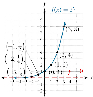
Let’s define the behavior of the graph of the exponential function [latex]f(x)=2^x[/latex] and highlight some its key characteristics.

• the domain is [latex](−∞,∞)[/latex],
• the range is [latex](0,∞)[/latex],
• as [latex]x→∞,f(x)→∞[/latex],
• as [latex]x→−∞,f(x)→0[/latex],
• [latex]f(x)[/latex] is always increasing,
• the graph of [latex]f(x)[/latex] will never touch the x-axis because base two raised to any exponent never has the result of zero.
• [latex]y=0[/latex] is the horizontal asymptote.
• the y-intercept is 1.

Evaluating Exponential Functions

Recall that the base of an exponential function must be a positive real number other than [latex]1[/latex]. Why do we limit the base [latex]b[/latex] to positive values? To ensure that the outputs will be real numbers. Observe what happens if the base is not positive:

• Let [latex]b=−9[/latex] and [latex]x=\frac{1}{2}[/latex]. Then [latex]f(x)=f(\frac{1}{2})=−9^{\frac{1}{2}}=\sqrt{−9},[/latex] which is not a real number.

Why do we limit the base to positive values other than [latex]1[/latex]? Because base [latex]1[/latex] results in the constant function. Observe what happens if the base is [latex]1[/latex]:

• Let [latex]b=1[/latex]. Then [latex]f(x)=1^x=1[/latex] for any value of [latex]x[/latex].

To evaluate an exponential function with the form [latex]f(x)=b^x[/latex], we simply substitute [latex]x[/latex] with the given value, and calculate the resulting power. For example:

Let [latex]f(x)=2^x[/latex]. What is [latex]f(3)[/latex]?

To evaluate an exponential function with a form other than the basic form, it is important to follow the order of operations. For example:

Let [latex]f(x)=30(2)^x[/latex]. What is [latex]f(3)[/latex]?

Note that if the order of operations were not followed, the result would be incorrect:

Defining Exponential Growth and Decay

Because the output of exponential functions increases or decreases very rapidly, the term “exponential growth” is often used to describe anything that grows or increases rapidly and the term “exponential decay” is used to describe anything that decays or decreases rapidly. However, exponential growth and decay can be defined more precisely in a mathematical sense. If the growth rate is proportional to the amount present, the function models exponential growth. Similarly, if the decay rate is proportional to the amount present, the function models exponential decay.

In more general terms, we have an exponential function, in which a constant base is raised to a variable exponent. To differentiate between linear and exponential functions, let’s consider two companies, A and B. Company A has 100 stores and expands by opening 50 new stores a year, so its growth can be represented by the function [latex]A(x)=100+50x[/latex]. Company B has 100 stores and expands by increasing the number of stores by 50% each year, so its growth can be represented by the function [latex]B(x)=100(1+0.5)^x[/latex].

A few years of growth for these companies are illustrated in Table 3.

The graphs comparing the number of stores for each company over a five-year period are shown in Figure 2. We can see that, with exponential growth, the number of stores increases much more rapidly than with linear growth.

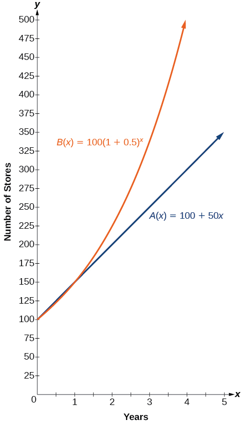
Notice that the domain for both functions is [latex][0,∞)[/latex], and the range for both functions is [latex][100,∞)[/latex]. After year 1, Company B always has more stores than Company A.

Now we will turn our attention to the function representing the number of stores for Company B, [latex]B(x)=100(1+0.5)^x[/latex]. In this exponential function, 100 represents the initial number of stores, 0.50 represents the growth rate, and [latex]1+0.5=1.5[/latex] represents the growth factor. Generalizing further, we can write this function as [latex]B(x)=100(1.5)^x[/latex], where 100 is the initial value, [latex]1.5[/latex] is called the base, and [latex]x[/latex] is called the exponent.

Finding Equations of Exponential Functions

In the previous examples, we were given an exponential function, which we then evaluated for a given input. Sometimes we are given information about an exponential function without knowing the function explicitly. We must use the information to first write the form of the function, then determine the constants [latex]a[/latex] and [latex]b[/latex], and evaluate the function.

Example 5

Writing an Exponential Model When the Initial Value Is Known

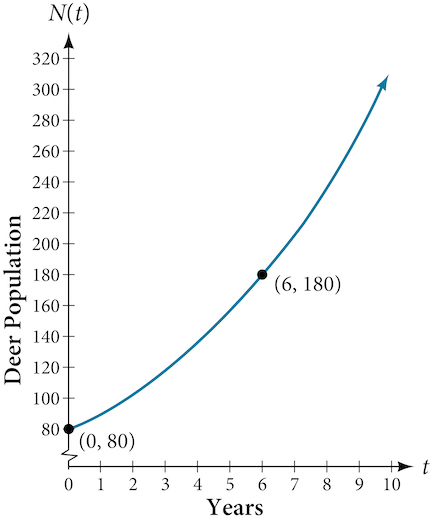
In 2006, 80 deer were introduced into a wildlife refuge. By 2012, the population had grown to 180 deer. The population was growing exponentially. Write an exponential function [latex]N(t)[/latex] representing the population [latex]N[/latex] of deer over time [latex]t[/latex].

 

Show/Hide Solution

Solution

We let our independent variable [latex]t[/latex] be the number of years after 2006. Thus, the information given in the problem can be written as input-output pairs: [latex](0, 80)[/latex] and [latex](6, 180)[/latex]. Notice that by choosing our input variable to be measured as years after 2006, we have given ourselves the initial value for the function, [latex]a=80[/latex]. We can now substitute the second point into the equation [latex]N(t)=80b^t[/latex] to find [latex]b[/latex]:

NOTE: Unless otherwise stated, do not round any intermediate calculations. Then round the final answer to four places for the remainder of this section.

The exponential model for the population of deer is [latex]N(t)=801.1447t[/latex]. (Note that this exponential function models short-term growth. As the inputs gets large, the output will get increasingly larger, so much so that the model may not be useful in the long term.)

We can graph our model to observe the population growth of deer in the refuge over time. Notice that the graph in Figure 3 passes through the initial points given in the problem, [latex](0,80)[/latex] and [latex](6,180)[/latex]. We can also see that the domain for the function is [latex][0,∞)[/latex], and the range for the function is [latex][80,∞)[/latex].

Example 6

Writing an Exponential Model When the Initial Value is Not Known

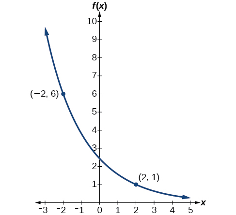
Find an exponential function that passes through the points [latex](−2,6)[/latex] and [latex](2,1)[/latex].

 

Show/Hide Solution

Solution

Because we don’t have the initial value, we substitute both points into an equation of the form [latex]f(x)=ab^x[/latex], and then solve the system for [latex]a[/latex] and [latex]b[/latex]. Substituting [latex](−2,6)[/latex] gives [latex]6=ab^{−2}[/latex]

Substituting [latex](2,1)[/latex] gives [latex]1=ab^2[/latex]

Use the first equation to solve for [latex]a[/latex] in terms of [latex]b[/latex]:

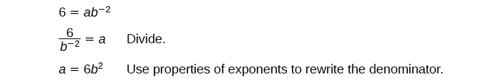
Substitute [latex]a[/latex] in the second equation, and solve for [latex]b[/latex]:

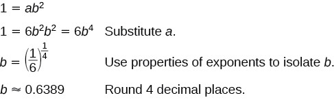
Use the value of [latex]b[/latex] in the first equation to solve for the value of [latex]a[/latex]:

Thus, the equation is [latex]f(x)=2.4492(0.6389)^x[/latex].

We can graph our model to check our work. Notice that the graph in Figure 4 passes through the initial points given in the problem, [latex](−2,6)[/latex] and [latex](2,1)[/latex]. The graph is an example of an exponential decay function.

Example 7

Writing an Exponential Function Given Its Graph

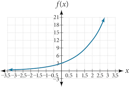
Find an equation for the exponential function graphed in Figure 5.

 

Show/Hide Solution

Solution

We can choose the y-intercept of the graph, [latex](0,3)[/latex], as our first point. This gives us the initial value, [latex]a=3[/latex]. Next, choose a point on the curve some distance away from [latex](0,3)[/latex] that has integer coordinates. One such point is [latex](2,12)[/latex].

Because we restrict ourselves to positive values of [latex]b[/latex], we will use [latex]b=2[/latex]. Substitute [latex]a[/latex] and [latex]b[/latex] into the standard form to yield the equation [latex]f(x)=3(2)^x[/latex].

Try It #6

Find an equation for the exponential function graphed in Figure 6.

Applying the Compound-Interest Formula

Savings instruments in which earnings are continually reinvested, such as mutual funds and retirement accounts, use compound interest. The term compounding refers to interest earned not only on the original value, but on the accumulated value of the account.

The annual percentage rate (APR) of an account, also called the nominal rate, is the yearly interest rate earned by an investment account. The term nominal is used when the compounding occurs a number of times other than once per year. In fact, when interest is compounded more than once a year, the effective interest rate ends up being greater than the nominal rate! This is a powerful tool for investing.

We can calculate the compound interest using the compound interest formula, which is an exponential function of the variables time [latex]t[/latex], principal [latex]P[/latex], APR [latex]r[/latex], and number of compounding periods in a year [latex]n[/latex]:

For example, observe Table 4, which shows the result of investing $1,000 at 10% for one year. Notice how the value of the account increases as the compounding frequency increases.

Evaluating Functions with Base e

As we saw earlier, the amount earned on an account increases as the compounding frequency increases. Table 5 shows that the increase from annual to semi-annual compounding is larger than the increase from monthly to daily compounding. This might lead us to ask whether this pattern will continue.

Examine the value of $1 invested at 100% interest for 1 year, compounded at various frequencies, listed in Table 5.

These values appear to be approaching a limit as [latex]n[/latex] increases without bound. In fact, as [latex]n[/latex] gets larger and larger, the expression [latex](1+\frac{1}{n})^n[/latex] approaches a number used so frequently in mathematics that it has its own name: the letter [latex]e[/latex]. This value is an irrational number, which means that its decimal expansion goes on forever without repeating. Its approximation to six decimal places is shown below.

Investigating Continuous Models

Now that we know how to represent [latex]e[/latex] as an irrational number, let’s see how this affects the compound interest formula we denoted earlier. Suppose that the number of compounding periods, [latex]n[/latex], increases indefinitely, if we let ,[latex]m=\frac{r}{n}[/latex], then

[latex]A(t)=P(1+\frac{r}{n})^{nt} = P[(1+\frac{r}{n})^{\frac{n}{r}}]^{rt} = P[(1+\frac{1}{m})^{m}]^{rt} = P(e)^{rt}[/latex]

This expression uses [latex]e[/latex] to give the amount when the interest is compounded at “every instant”. Interestingly, for most real-world phenomena, [latex]e[/latex] is used as the base for exponential functions. Exponential models that use [latex]e[/latex] as the base are called continuous compound interest or continuous growth/decay. We see these models in finance, computer science, and most of the sciences, such as physics, toxicology, and fluid dynamics.

Graphs of Exponential Functions

As we discussed above, exponential functions are used for many real-world applications such as finance, forensics, computer science, and most of the life sciences. Working with an equation that describes a real-world situation gives us a method for making predictions. Most of the time, however, the equation itself is not enough. We learn a lot about things by seeing their pictorial representations, and that is exactly why graphing exponential equations is a powerful tool. It gives us another layer of insight for predicting future events.

Graphing Exponential Functions

Before we begin graphing, it is helpful to review the behavior of exponential growth. Recall the table of values for a function of the form [latex]f(x)=b^x[/latex] whose base is greater than one. We’ll use the function [latex]f(x)=2^x[/latex]. Observe how the output values in Table 6 change as the input increases by [latex]1[/latex].

Table 6

[latex]x[/latex]	[latex]−3[/latex]	[latex]−2[/latex]	[latex]−1[/latex]	[latex]0[/latex]	[latex]1[/latex]	[latex]2[/latex]	[latex]3[/latex]
[latex]f(x)=2^x[/latex]	[latex]18[/latex]	[latex]14[/latex]	[latex]12[/latex]	[latex]1[/latex]	[latex]2[/latex]	[latex]4[/latex]	[latex]8[/latex]

Each output value is the product of the previous output and the base, [latex]2[/latex]. We call the base [latex]2[/latex] the constant ratio. In fact, for any exponential function with the form [latex]f(x)=ab^x[/latex], [latex]b[/latex] is the constant ratio of the function. This means that as the input increases by 1, the output value will be the product of the base and the previous output, regardless of the value of [latex]a[/latex].

Notice from the table that

• the output values are positive for all values of [latex]x[/latex];
• as [latex]x[/latex] increases, the output values increase without bound; and
• as [latex]x[/latex] decreases, the output values grow smaller, approaching zero.

Figure 7 shows the exponential growth function [latex]f(x)=2^x[/latex].

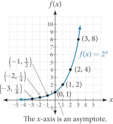
The domain of [latex]f(x)=2^x[/latex] is all real numbers, the range is [latex](0,∞)[/latex], and the horizontal asymptote is [latex]y=0[/latex].

To get a sense of the behavior of exponential decay, we can create a table of values for a function of the form [latex]f(x)=b^x[/latex] whose base is between zero and one. We’ll use the function [latex]g(x)=(\frac{1}{2})^x[/latex]. Observe how the output values in Table 7 change as the input increases by [latex]1[/latex].

Table 7

[latex]x[/latex]	[latex]−3[/latex]	[latex]−2[/latex]	[latex]−1[/latex]	[latex]0[/latex]	[latex]1[/latex]	[latex]2[/latex]	[latex]3[/latex]
[latex]g(x)=(\frac{1}{2})^x[/latex]	[latex]8[/latex]	[latex]4[/latex]	[latex]2[/latex]	[latex]1[/latex]	[latex]\frac{1}{2}[/latex]	[latex]\frac{1}{4}[/latex]	[latex]\frac{1}{8}[/latex]

Again, because the input is increasing by 1, each output value is the product of the previous output and the base, or constant ratio [latex]\frac{1}{2}[/latex].

Notice from the table that:

• the output values are positive for all values of [latex]x[/latex];
• as [latex]x[/latex] increases, the output values grow smaller, approaching zero; and
• as [latex]x[/latex] decreases, the output values grow without bound.

Figure 8 shows the exponential decay function, [latex]g(x)=(\frac{1}{2})^x[/latex].

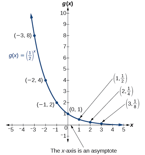
The domain of [latex]g(x)=(\frac{1}{2})^x[/latex] is all real numbers, the range is [latex](0,∞)[/latex], and the horizontal asymptote is [latex]y=0[/latex].

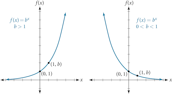
Characteristics of the Graph of the Exponential Parent Function

An exponential function with the form [latex]f(x)=b^x[/latex], [latex]b>0[/latex], [latex]b≠1[/latex], has these characteristics:

• one-to-one function
• horizontal asymptote: [latex]y=0[/latex]
• domain: [latex](–∞, ∞)[/latex]
• range: [latex](0,∞)[/latex]
• x-intercept: none
• y-intercept: [latex](0,1)[/latex]
• increasing if [latex]b>1[/latex]
• decreasing if [latex]b<1[/latex]

Figure 9 compares the graphs of exponential growth and decay functions.

How To

Given an exponential function of the form f(x) = b^x, graph the function.

1. Create a table of points.
2. Plot at least [latex]3[/latex] point from the table, including the y-intercept [latex](0,1)[/latex].
3. Draw a smooth curve through the points.
4. State the domain, [latex](−∞,∞)[/latex], the range, [latex](0,∞)[/latex], and the horizontal asymptote, [latex]y=0[/latex].

Example 12

Sketching the Graph of an Exponential Function of the Form f(x) = b^x

Sketch a graph of [latex]f(x)=0.25^x[/latex]. State the domain, range, and asymptote.

 

Show/Hide Solution

Solution

Before graphing, identify the behavior and create a table of points for the graph.

• Since [latex]b=0.25[/latex] is between zero and one, we know the function is decreasing. The left tail of the graph will increase without bound, and the right tail will approach the asymptote [latex]y=0[/latex].
• Create a table of points as in Table 8.

Table 8

[latex]x[/latex]	[latex]−3[/latex]	[latex]−2[/latex]	[latex]−1[/latex]	[latex]0[/latex]	[latex]1[/latex]	[latex]2[/latex]	[latex]3[/latex]
[latex]f(x)=0.25^x[/latex]	[latex]64[/latex]	[latex]16[/latex]	[latex]4[/latex]	[latex]1[/latex]	[latex]0.25[/latex]	[latex]0.0625[/latex]	[latex]0.015625[/latex]

• Plot the y-intercept, [latex](0,1)[/latex], along with two other points. We can use [latex](−1,4)[/latex] and [latex](1,0.25)[/latex].

Draw a smooth curve connecting the points as in Figure 10.

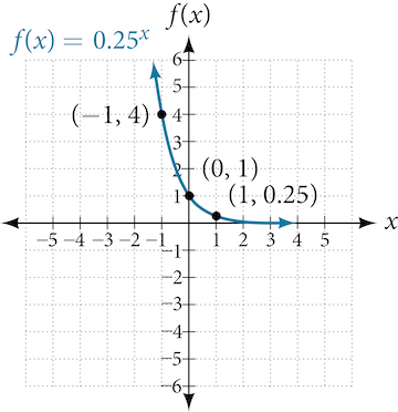
The domain is [latex](−∞,∞)[/latex]; the range is [latex](0,∞)[/latex]; the horizontal asymptote is [latex]y=0[/latex].

Try It #11

Sketch the graph of [latex]f(x)=4^x[/latex]. State the domain, range, and asymptote.

Graphing Transformations of Exponential Functions

Transformations of exponential graphs behave similarly to those of other functions. Just as with other parent functions, we can apply the four types of transformations—shifts, reflections, stretches, and compressions—to the parent function [latex]f(x)=b^x[/latex] without loss of shape. For instance, just as the quadratic function maintains its parabolic shape when shifted, reflected, stretched, or compressed, the exponential function also maintains its general shape regardless of the transformations applied.

Graphing a Vertical Shift

The first transformation occurs when we add a constant [latex]d[/latex] to the parent function [latex]f(x)=b^x[/latex], giving us a vertical shift [latex]d[/latex] units in the same direction as the sign. For example, if we begin by graphing a parent function, [latex]f(x)=2^x[/latex], we can then graph two vertical shifts alongside it, using [latex]d=3[/latex]: the upward shift, [latex]g(x)=2^x+3[/latex] and the downward shift, [latex]h(x)=2^x−3[/latex]. Both vertical shifts are shown in Figure 11.

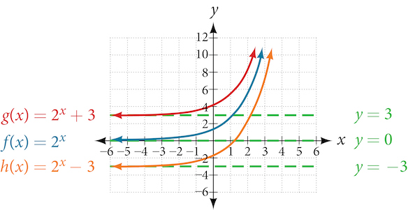
Observe the results of shifting [latex]f(x)=2^x[/latex] vertically:

• The domain, (−∞,∞) remains unchanged.
• When the function is shifted up [latex]3[/latex] units to [latex]g(x)=2^x+3[/latex]:
  • The y-intercept shifts up [latex]3[/latex] units to [latex](0,4)[/latex].
  • The asymptote shifts up [latex]3[/latex] units to [latex]y=3[/latex].
  • The range becomes [latex](3,∞)[/latex].
• When the function is shifted down [latex]3[/latex] units to [latex]h(x)=2^x−3[/latex]:
  • The y-intercept shifts down [latex]3[/latex] units to [latex](0,−2)[/latex].
  • The asymptote also shifts down [latex]3[/latex] units to [latex]y=−3[/latex].
  • The range becomes [latex](−3,∞)[/latex].

Graphing a Horizontal Shift

The next transformation occurs when we add a constant [latex]c[/latex] to the input of the parent function [latex]f(x)=b^x[/latex], giving us a horizontal shift [latex]c[/latex] units in the opposite direction of the sign. For example, if we begin by graphing the parent function [latex]f(x)=2^x[/latex], we can then graph two horizontal shifts alongside it, using [latex]c=3[/latex]: the shift left, [latex]g(x)=2^{x+3}[/latex], and the shift right, [latex]h(x)=2^{x−3}[/latex]. Both horizontal shifts are shown in Figure 12.

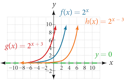
Observe the results of shifting [latex]f(x)=2^x[/latex] horizontally:

• The domain, [latex](−∞,∞)[/latex], remains unchanged.
• The asymptote, [latex]y=0[/latex], remains unchanged.
• The y-intercept shifts such that:
  • When the function is shifted left [latex]3[/latex] units to [latex]g(x)=2^{x+3}[/latex], the y-intercept becomes [latex](0,8)[/latex]. This is because [latex]2^{x+3}=(8)2^x[/latex], so the initial value of the function is [latex]8[/latex].
  • When the function is shifted right [latex]3[/latex] units to [latex]h(x)=2^{x−3}[/latex], the y-intercept becomes [latex](0,\frac{1}{8})[/latex]. Again, see that [latex]2^{x−3}=(\frac{1}{8})2^x[/latex], so the initial value of the function is [latex]\frac{1}{8}[/latex].

Graphing a Stretch or Compression

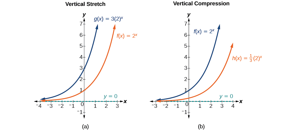
While horizontal and vertical shifts involve adding constants to the input or to the function itself, a stretch or compression occurs when we multiply the parent function [latex]f(x)=b^x[/latex] by a constant [latex]|a|>0[/latex]. For example, if we begin by graphing the parent function [latex]f(x)=2^x[/latex], we can then graph the stretch, using [latex]a=3[/latex], to get [latex]g(x)=3(2)^x[/latex] as shown on the left in Figure 13, and the compression, using [latex]a=\frac{1}{3}[/latex], to get [latex]h(x)=\frac{1}{3}(2)^x[/latex] as shown on the right in Figure 13.

Graphing Reflections

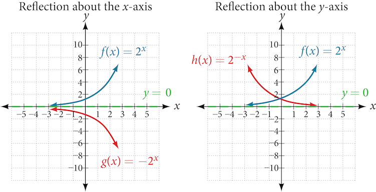
In addition to shifting, compressing, and stretching a graph, we can also reflect it about the x-axis or the y-axis. When we multiply the parent function [latex]f(x)=b^x[/latex] by [latex]−1[/latex], we get a reflection about the x-axis. When we multiply the input by [latex]−1[/latex], we get a reflection about the y-axis. For example, if we begin by graphing the parent function [latex]f(x)=2^x[/latex], we can then graph the two reflections alongside it. The reflection about the x-axis, [latex]g(x)=−2^x[/latex], is shown on the left side of Figure 14, and the reflection about the y-axis [latex]h(x)=2^{−x}[/latex], is shown on the right side of Figure 14.

Summarizing Translations of the Exponential Function

Now that we have worked with each type of translation for the exponential function, we can summarize them in Table 9 to arrive at the general equation for translating exponential functions.

Table 9

Transformations of the Parent Function [latex]f(x)=b^x[/latex]
Transformation	Form
Shift Horizontally [latex]c[/latex] units to the left Vertically [latex]d[/latex] units up	[latex]f(x)=b^{x+c}+d[/latex]
Stretch and Compress Stretch if [latex]|a|>1[/latex] Compression if [latex]0<|a|<1[/latex]	[latex]f(x)=ab^x[/latex]
Reflect about the x-axis	[latex]f(x)=−b^x[/latex]
Reflect about the y-axis	[latex]f(x)=b^{−x}=(\frac{1}{b})^x[/latex]
General equation for all translations	[latex]f(x)=ab^{x+c}+d[/latex]

Translations of Exponential Functions

A translation of an exponential function has the form

[latex] f(x)=ab^{x+c}+d[/latex]

Where the parent function, [latex]y=b^x[/latex], [latex]b>1[/latex], is

• shifted horizontally [latex]c[/latex] units to the left.
• stretched vertically by a factor of [latex]|a|[/latex] if [latex]|a|>0[/latex].
• compressed vertically by a factor of [latex]|a|[/latex] if [latex]0<|a|<1[/latex].
• shifted vertically [latex]d[/latex] units.
• reflected about the x-axis when [latex]a<0[/latex].

Note the order of the shifts, transformations, and reflections follow the order of operations.

Characteristics of the Graph of Translations of the Exponential Parent Function

An exponential function with the form [latex]f(x)=ab^{x+c}+d[/latex], [latex]b>0[/latex], [latex]b≠1[/latex], has these characteristics:

• one-to-one function
• horizontal asymptote: [latex]y=d[/latex]
• domain: [latex](–∞, ∞)[/latex], remains unchanged
• range: [latex](d,∞)[/latex]
• x-intercept: [latex](log_b(\frac{–d}{a})–c ,0)[/latex]
• y-intercept: [latex](0,a(b^c)+d)[/latex]
• increasing if [latex]b>1[/latex]
• decreasing if [latex]b<1[/latex]

Example 13

Writing a Function from a Description

Write the equation for the function described below. Give the horizontal asymptote, the domain, and the range. [latex]f(x)=e^x[/latex] is vertically stretched by a factor of [latex]2[/latex], reflected across the y-axis, and then shifted up [latex]4[/latex] units.

 

Show/Hide Solution

Solution

We want to find an equation of the general form [latex]f(x)=ab^{x+c}+d[/latex].

We use the description provided to find [latex]a[/latex], [latex]b[/latex], [latex]c[/latex], and [latex]d[/latex].

• We are given the parent function [latex]f(x)=e^x[/latex], so [latex]b=e[/latex].
• The function is stretched by a factor of [latex]2[/latex], so [latex]a=2[/latex].
• The function is reflected about the y-axis. We replace [latex]x[/latex] with [latex]−x[/latex] to get: [latex]e^{−x}[/latex].
• The graph is shifted vertically 4 units, so [latex]d=4[/latex].

Substituting in the general form we get,

The domain is [latex](−∞,∞)[/latex]; the range is [latex](4,∞)[/latex]; the horizontal asymptote is [latex]y=4[/latex].

Try It #12

Write the equation for function described below. Give the horizontal asymptote, the domain, and the range. [latex]f(x)=e^x[/latex] is compressed vertically by a factor of [latex]\frac{1}{3}[/latex], reflected across the x-axis and then shifted down [latex]2[/latex] units.

Media

Access these online resources for additional instruction and practice with exponential functions.

• Exponential Growth Function
• Compound Interest
• Graph Exponential Functions

Section Exercises

Verbal

1. Explain why the values of an increasing exponential function will eventually overtake the values of an increasing linear function.

2. Given a formula for an exponential function, is it possible to determine whether the function grows or decays exponentially just by looking at the formula? Explain.

3. What role does the horizontal asymptote of an exponential function play in telling us about the end behavior of the graph?

Algebraic

For the following exercises, identify whether the statement represents an exponential function. Explain.

4. The average annual population increase of a pack of wolves is 25.

5. A population of bacteria decreases by a factor of [latex]\frac{1}{8}[/latex] every [latex]24[/latex] hours.

6. Height of a projectile at time [latex]t[/latex] is represented by the function [latex]h(t)=−4.9t^2+18t+40[/latex].

For the following exercises, consider this scenario: For each year [latex]t[/latex], the population of a forest of trees is represented by the function [latex]A(t)=115(1.025)^t[/latex]. In a neighboring forest, the population of the same type of tree is represented by the function [latex]B(t)=82(1.029)^t[/latex]. (Round answers to the nearest whole number.)

7. Which forest’s population is growing at a faster rate?

8. Which forest had a greater number of trees initially? By how many?

9. Assuming the population growth models continue to represent the growth of the forests, which forest will have a greater number of trees after [latex]20[/latex] years? By how many?

10. Assuming the population growth models continue to represent the growth of the forests, which forest will have a greater number of trees after [latex]100[/latex] years? By how many?

For the following exercises, determine whether the equation represents exponential growth, exponential decay, or neither. Explain.

11. [latex]y=220(1.06)^x[/latex]

12. [latex]y=300(1−t)^5[/latex]

For the following exercises, find the formula for an exponential function that passes through the two points given.

13. [latex](0,2000)[/latex] and [latex](2,20)[/latex]

14. [latex](−2,6)[/latex] and [latex](3,1)[/latex]

For the following exercises, determine whether the table could represent a function that is linear, exponential, or neither. If it appears to be exponential, find a function that passes through the points.

15.

16.

For the following exercises, use the compound interest formula, [latex]A(t)=P(1+\frac{r}{n})^{nt}[/latex].

17. After a certain number of years, the value of an investment account is represented by the equation [latex]A=10,250(1+\frac{0.04}{12})^{120}[/latex]. What is the value of the account?

18. What was the initial deposit made to the account in the previous exercise?

19. How many years had the account from the previous exercise been accumulating interest?

For the following exercises, determine whether the equation represents continuous growth, continuous decay, or neither. Explain.

20. [latex]y=3742(e)^{0.75t}[/latex]

21. [latex]y=2.25(e)^{−2t}[/latex]

For the following exercises, graph the function given its translations, then state the new equation, y-intercept, domain, and range.

22. The graph of [latex]f(x)=(\frac{1}{2})^{−x}[/latex] is reflected about the y-axis and compressed vertically by a factor of [latex]\frac{1}{5}[/latex]. What is the equation of the new function, [latex]g(x)[/latex]? State its y-intercept, domain, and range.

23. The graph of [latex]f(x)=3^x[/latex] is reflected about the y-axis and stretched vertically by a factor of [latex]4[/latex]. What is the equation of the new function, [latex]g(x)[/latex]? State its y-intercept, domain, and range.

24. The graph of [latex]f(x)=−\frac{1}{2}(\frac{1}{4})^{x−2}+4[/latex] is shifted downward [latex]4[/latex] units, and then shifted left [latex]2[/latex] units, stretched vertically by a factor of [latex]4[/latex], and reflected about the x-axis. What is the equation of the new function, [latex]g(x)[/latex]? State its y-intercept, domain, and range.

Graphical

For the following exercises, graph the function and its reflection about the y-axis on the same axes, and give the y-intercept.

25. [latex]g(x)=−2(0.25)^x[/latex]

26. [latex]h(x)=3(\frac{1}{2})^x[/latex]

For the following exercises, match each function with one of the graphs in Figure 15.

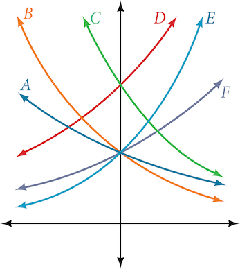
27. [latex]f(x)=2(0.69)^x[/latex]

28. [latex]f(x)=2(1.28)^x[/latex]

29. [latex]f(x)=2(0.81)^x[/latex]

30. [latex]f(x)=4(1.28)^x[/latex]

31. [latex]f(x)=2(1.59)^x[/latex]

32. [latex]f(x)=4(0.69)^x[/latex]

For the following exercises, use the graphs shown in Figure 16. All have the form [latex]f(x)=ab^x[/latex].

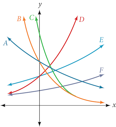
33. Which graph has the largest value for [latex]b[/latex]?

34. Which graph has the largest value for [latex]a[/latex]?

For the following exercises, describe the end behavior of the graphs of the functions.

35. [latex]f(x)=−5(4)^x−1[/latex]

36. [latex]f(x)=3(\frac{1}{2})^x−2[/latex]

37. [latex]f(x)=3(4)^{−x}+2[/latex]

For the following exercises, graph the transformation of [latex]f(x)=2^x[/latex]. Give the horizontal asymptote, the domain, and the range.

38. [latex]f(x)=2^{−x}[/latex]

39. [latex]h(x)=2^x+3[/latex]

40. [latex]f(x)=2^{x−2}[/latex]

For the following exercises, start with the graph of [latex]f(x)=4^x[/latex]. Then write a function that results from the given transformation.

41. Shift [latex]f(x)[/latex] 4 units upward

42. Shift [latex]f(x)[/latex] 5 units right

43. Reflect [latex]f(x)[/latex] about the x-axis

44. Reflect [latex]f(x)[/latex] about the y-axis

For the following exercises, each graph is a transformation of [latex]y=2^x[/latex]. Write an equation describing the transformation.

45.

46.

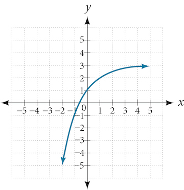
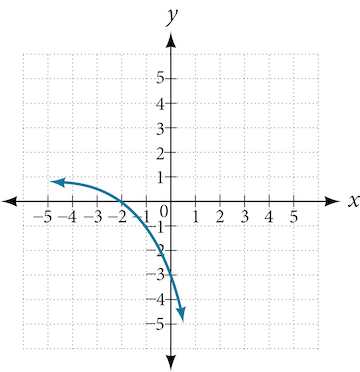
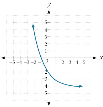
For the following exercises, find an exponential equation for the graph.

47.

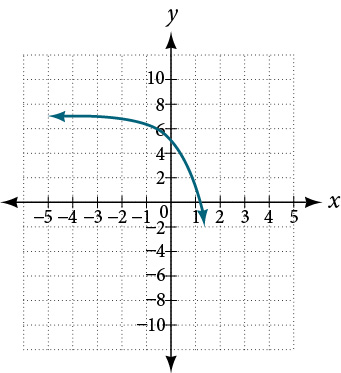
48.

Numeric

For the following exercises, evaluate each function. Round answers to four decimal places, if necessary.

49. [latex]f(x)=−4^{2x+3}[/latex], for [latex]f(−1)[/latex]

50. [latex]f(x)=−\frac{3}{2}(3)^{−x}+\frac{3}{2}[/latex], for [latex]f(2)[/latex]

51. [latex]f(x)=−2e^{x−1}[/latex], for [latex]f(−1)[/latex]

For the following exercises, evaluate the exponential functions for the indicated value of [latex]x[/latex].

52. [latex]g(x)=\frac{1}{3}(7)^{x−2}[/latex] for [latex]g(6)[/latex].

53. [latex]h(x)=−\frac{1}{2}(\frac{1}{2})^x+6[/latex] for [latex]h(−7)[/latex].

Extensions

54. Recall that an exponential function is any equation written in the form [latex]f(x)=a⋅b^x[/latex] such that [latex]a[/latex] and [latex]b[/latex] are positive numbers and [latex]b≠1[/latex]. Any positive number [latex]b[/latex] can be written as [latex]b=e^n[/latex] for some value of [latex]n[/latex]. Use this fact to rewrite the formula for an exponential function that uses the number [latex]e[/latex]  as a base.

55. In an exponential decay function, the base of the exponent is a value between 0 and 1. Thus, for some number [latex]b>1[/latex], the exponential decay function can be written as [latex]f(x)=a⋅(\frac{1}{b})x[/latex]. Use this formula, along with the fact that [latex]b=e^n[/latex], to show that an exponential decay function takes the form [latex]f(x)=a(e)^{−nx}[/latex] for some positive number [latex]n[/latex].

56. Explore and discuss the graphs of [latex]F(x)=(b)^x[/latex] and [latex]G(x)=(\frac{1}{b})^x[/latex]. Then make a conjecture about the relationship between the graphs of the functions [latex](b)^x[/latex] and [latex](\frac{1}{b})^x[/latex] for any real number [latex]b>0[/latex].

57. Explore and discuss the graphs of [latex]f(x)=4^x[/latex], [latex]g(x)=4^{x−2}[/latex], and [latex]h(x)=(\frac{1}{16})4^x[/latex]. Then make a conjecture about the relationship between the graphs of the functions [latex]b^x[/latex] and [latex](\frac{1}{b^n})b^x[/latex] for any real number n and real number [latex]b>0[/latex].

Real-World Applications

58. A scientist begins with 100 milligrams of a radioactive substance that decays exponentially. After 35 hours, 50mg of the substance remains. How many milligrams will remain after 54 hours?

59. The fox population in a certain region has an annual growth rate of 9% per year. In the year 2012, there were 23,900 fox counted in the area. What is the fox population predicted to be in the year 2020?

60. A car was valued at $38,000 in the year 2007. By 2013, the value had depreciated to $11,000 If the car’s value continues to drop by the same percentage, what will it be worth by 2017?

61. In the year 1985, a house was valued at $110,000. By the year 2005, the value had appreciated to $145,000. What was the annual growth rate between 1985 and 2005? Assume that the value continued to grow by the same percentage. What was the value of the house in the year 2010?

62. Jaylen wants to save $54,000 for a down payment on a home. How much will he need to invest in an account with 8.2% APR, compounding daily, in order to reach his goal in 5 years?