Chapter 5 – Further Applications of Trigonometry
“Try It” Exercises
Section 5.1 – Non-right Triangles: Law of Sines
1.

2. Solution 1

Solution 2

3. [latex]β≈5.7∘,γ≈94.3∘,c≈101.3[/latex]
4. two
5. about [latex]8.2[/latex] square feet
6. 161.9 yd.
Section 5.2 – Non-right Triangles: Law of Cosines
1. [latex]a≈14.9[/latex],
[latex]β≈23.8∘[/latex],
[latex]γ≈126.2∘[/latex].
2. [latex]α≈27.7∘[/latex],
[latex]β≈40.5∘[/latex],
[latex]γ≈111.8∘[/latex]
3. Area = 552 square feet
4. about 8.15 square feet
Section 5.3 – Polar Coordinates
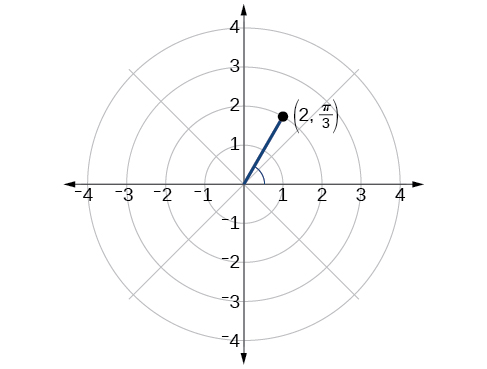
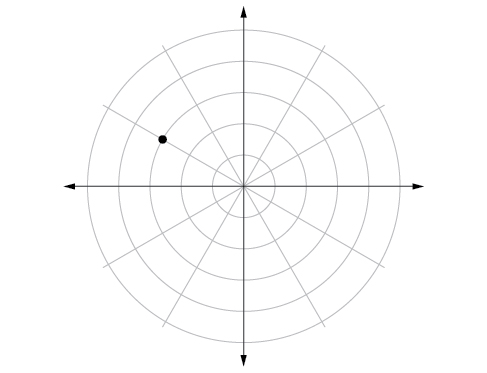
1.
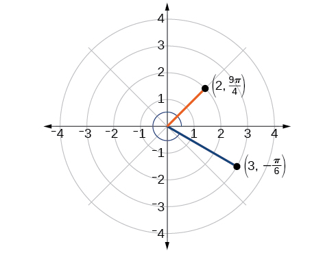
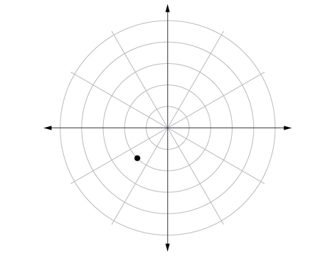
2.
3. [latex](x,y)=(\frac{1}{2},−\frac{\sqrt{3}}{2})[/latex]
4. [latex]r=3[/latex]
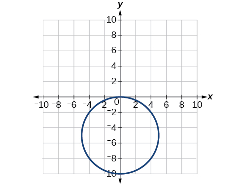
5. [latex]x^2+y^2=2y[/latex] or, in the standard form for a circle, [latex]x^2+(y−1)^2=1[/latex]
Section 5.4 – Polar Coordinates: Graphs
1. The equation fails the symmetry test with respect to the line [latex]θ=\frac{π}{2}[/latex] and with respect to the pole. It passes the polar axis symmetry test.
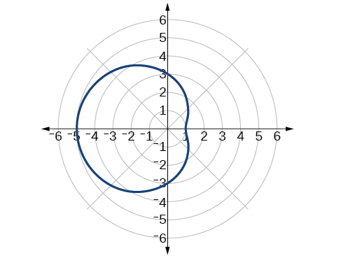
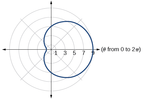
2. Tests will reveal symmetry about the polar axis. The zero is [latex](0,\frac{π}{2})[/latex], and the maximum value is [latex](3,0)[/latex].
3.
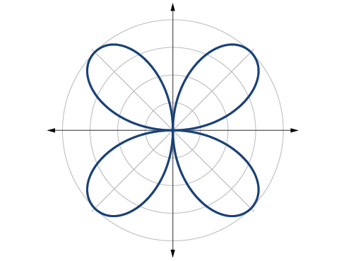
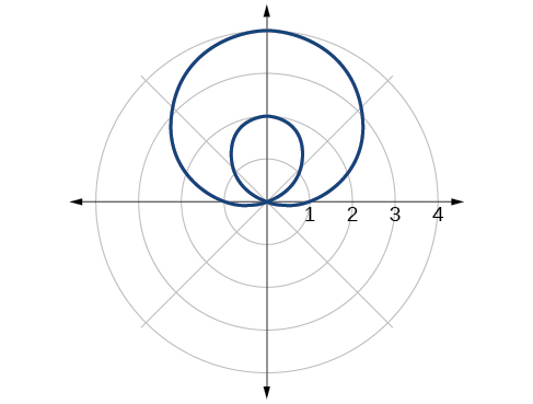
4. The graph is a rose curve, [latex]n[/latex] even
5.
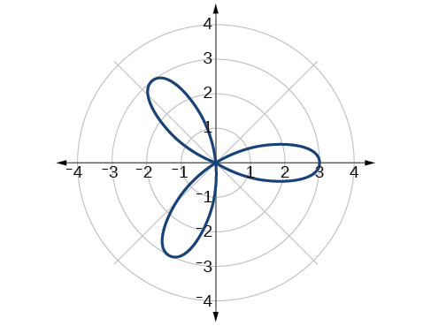
Rose curve, [latex]n[/latex] odd
6.
Section 5.5 – Polar Form of Complex Numbers
1.
2. 13
3. [latex]|z|=\sqrt{50}=5\sqrt{2}[/latex]
4. [latex]z=3(cos\frac{π}{2}+isin\frac{π}{2})[/latex]
5. [latex]z=2(cos\frac{π}{6}+isin\frac{π}{6})[/latex]
6. [latex]z=2\sqrt{3}−2i[/latex]
7. [latex]z_1z_2=−4\sqrt{3}; \frac{z_1}{z_2}=−\frac{\sqrt{3}}{2}+\frac{3}{2}i[/latex]
8. [latex]z_0=2(cos(30∘)+isin(30∘))[/latex]
[latex]z_1=2(cos(120∘)+isin(120∘))[/latex]
[latex]z_2=2(cos(210∘)+isin(210∘))[/latex]
[latex]z_3=2(cos(300∘)+isin(300∘))[/latex]
Section Exercises
Section 5.1 – Non-right Triangles: Law of Sines
1. The altitude extends from any vertex to the opposite side or to the line containing the opposite side at a 90° angle.
3. When the known values are the side opposite the missing angle and another side and its opposite angle.
5. A triangle with two given sides and a non-included angle.
7. [latex]β=72∘,a≈12.0,b≈19.9[/latex]
9. [latex]γ=20∘,b≈4.5,c≈1.6[/latex]
11. [latex]b≈3.78[/latex]
13. [latex]c≈13.70[/latex]
15. one triangle, [latex]α≈50.3∘,β≈16.7∘,a≈26.7[/latex]
17. two triangles, [latex]γ≈54.3∘,β≈90.7∘,b≈20.9[/latex] or [latex]γ′≈125.7∘,β′≈19.3∘,b′≈6.9[/latex]
19. two triangles, [latex]β≈75.7∘, γ≈61.3∘,b≈9.9[/latex] or [latex]β′≈18.3∘,γ′≈118.7∘,b′≈3.2[/latex]
21. two triangles, [latex]α≈143.2∘,β≈26.8∘,a≈17.3[/latex] or [latex]α′≈16.8∘,β′≈153.2∘,a′≈8.3[/latex]
23. no triangle possible
25. [latex]A≈47.8∘[/latex] or [latex]A′≈132.2∘[/latex]
27. [latex]8.6[/latex]
29. [latex]370.9[/latex]
31. [latex]12.3[/latex]
33. [latex]12.2[/latex]
35. [latex]16.0[/latex]
37. [latex]29.7∘[/latex]
39. [latex]x=76.9∘or x=103.1∘[/latex]
41. [latex]110.6∘[/latex]
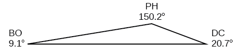
43. [latex]A≈39.4, C≈47.6, BC≈20.7[/latex]
45. [latex]57.1[/latex]
47. [latex]42.0[/latex]
49. [latex]430.2[/latex]
51. [latex]10.1[/latex]
53. [latex]AD≈ 13.8[/latex]
55. [latex]AB≈2.8[/latex]
57. [latex]L≈49.7, N≈56.3, LN≈5.8[/latex]
59. 51.4 feet
61. The distance from the satellite to station [latex]A[/latex] is approximately 1716 miles. The satellite is approximately 1706 miles above the ground.
63. 2.6 ft
65. 5.6 km
67. 371 ft
69. 5936 ft
71. 24.1 ft
73. 19,056 ft2
75. 445,624 square miles
77. 8.65 ft2
Section 5.2 – Non-right Triangles: Law of Cosines
1. two sides and the angle opposite the missing side.
3. [latex]s[/latex] is the semi-perimeter, which is half the perimeter of the triangle.
5. The Law of Cosines must be used for any oblique (non-right) triangle.
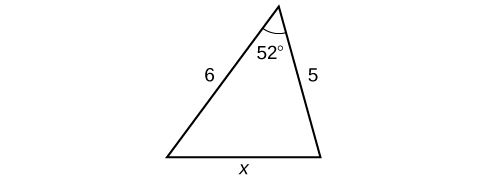
7. 11.3
9. 34.7
11. 26.7
13. c= 257.3, 96.7
15. not possible
17. 95.5°
19. 26.9°
21. [latex]B≈45.9∘,C≈99.1∘,a≈6.4[/latex]
23. [latex]A≈20.6∘,B≈38.4∘,c≈51.1[/latex]
25. [latex]A≈37.8∘,B≈43.8,C≈98.4∘[/latex]
27. 177.56 in2
29. 0.04 m2
31. 0.91 yd2
33. 3.0
35. 29.1
37. 0.5
39. 70.7°
41. 77.4°
43. 25.0
45. 9.3
47. 43.52
49. 1.41
51. 0.14
53. 18.3
54. 48.98
56.
58. 7.62
60. 85.1
62. 24.0 km
64. 99.9 ft
66. 37.3 miles
68. 2371 miles
70.
72. 292.4 miles
74. 65.4 cm2
76. 468 ft2
Section 5.3 – Polar Coordinates
1. For polar coordinates, the point in the plane depends on the angle from the positive x-axis and distance from the origin, while in Cartesian coordinates, the point represents the horizontal and vertical distances from the origin. For each point in the coordinate plane, there is one representation, but for each point in the polar plane, there are infinite representations.
3. Determine [latex]θ[/latex] for the point, then move [latex]r[/latex] units from the pole to plot the point. If [latex]r[/latex] is negative, move [latex]r[/latex] units from the pole in the opposite direction but along the same angle. The point is a distance of [latex]r[/latex] away from the origin at an angle of [latex]θ[/latex] from the polar axis.
5. The point [latex](−3,\frac{π}{2})[/latex] has a positive angle but a negative radius and is plotted by moving to an angle of [latex]\frac{π}{2}[/latex] and then moving 3 units in the negative direction. This places the point 3 units down the negative y-axis. The point [latex](3,−\frac{π}{2})[/latex] has a negative angle and a positive radius and is plotted by first moving to an angle of [latex]−\frac{π}{2}[/latex] and then moving 3 units down, which is the positive direction for a negative angle. The point is also 3 units down the negative y-axis.
7. [latex](−5,0)[/latex]
9. [latex](−\frac{3\sqrt{3}}{2},−\frac{3}{2})[/latex]
11. [latex](2\sqrt{5}, 0.464)[/latex]
13. [latex](\sqrt{34},5.253)[/latex]
15. [latex](8\sqrt{2},\frac{π}{4})[/latex]
17. [latex]r=4cscθ[/latex]
19. [latex]r=\sqrt[3]{\frac{sinθ}{2cos^4θ}}[/latex]
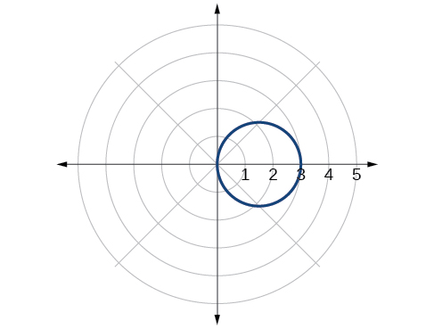
21. [latex]r=3cosθ[/latex]
23. [latex]r=\frac{3sinθ}{cos(2θ)}[/latex]
25. [latex]r=\frac{9sinθ}{cos^2θ}[/latex]
27. [latex]r=\sqrt{\frac{1}{9cosθsinθ}}[/latex]
29. [latex]x^2+y^2=4x[/latex] or [latex]\frac{(x−2)^2}{4}+\frac{y^2}{4}=1;[/latex] circle
31. [latex]3y+x=6;[/latex] line
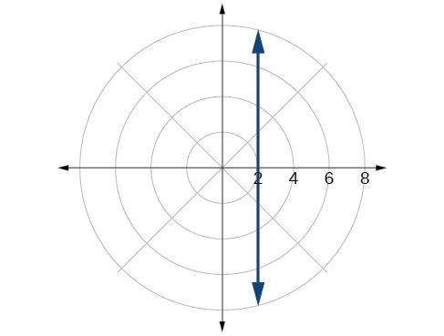
33. [latex]y=3;[/latex] line
35. [latex]xy=4;[/latex] hyperbola
37. [latex]x^2+y^2=4;[/latex] circle
39. [latex]x−5y=3;[/latex] line
41. [latex](3,\frac{3π}{4})[/latex]
43. [latex](5,π)[/latex]
45.
47.
49.
51.
53.
55. [latex]r=\frac{6}{5cosθ−sinθ}[/latex]
57. [latex]r=2sinθ[/latex]
59. [latex]r=\frac{2}{cosθ}[/latex]
61. [latex]r=3cosθ[/latex]
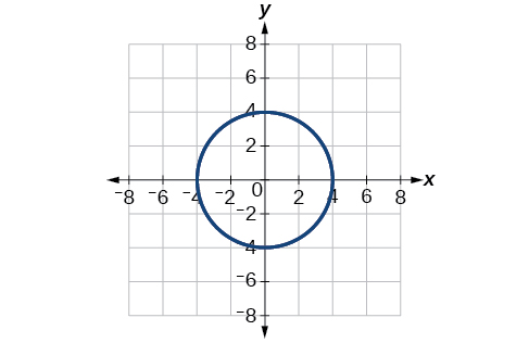
63. [latex]x^2+y^2=16[/latex]
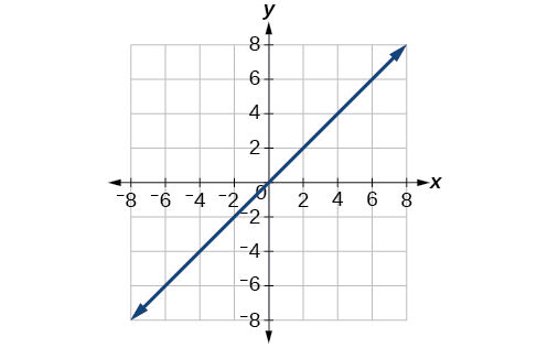
65. [latex]y=x[/latex]
67. [latex]x^2+(y+5)^2=25[/latex]
69. [latex](1.618,−1.176)[/latex]
71. [latex](10.630,131.186∘)[/latex]
73. [latex](2,3.14)[/latex] or [latex](2,π)[/latex]
75. A vertical line with [latex]a[/latex] units left of the y-axis.
77. A horizontal line with [latex]a[/latex] units below the x-axis.
79.
81.
83.
Section 5.4 – Polar Coordinates: Graphs
1. Symmetry with respect to the polar axis is similar to symmetry about the [latex]x[/latex]
-axis, symmetry with respect to the pole is similar to symmetry about the origin, and symetric with respect to the line [latex]θ=\frac{π}{2}[/latex] is similar to symmetry about the [latex]y[/latex]-axis.
3. Test for symmetry; find zeros, intercepts, and maxima; make a table of values. Decide the general type of graph, cardioid, limaçon, lemniscate, etc., then plot points at [latex]θ=0, \frac{π}{2}[/latex], [latex]π[/latex] and [latex]\frac{3π}{2}[/latex], and sketch the graph.
5. The shape of the polar graph is determined by whether or not it includes a sine, a cosine, and constants in the equation.
7. symmetric with respect to the polar axis
9. symmetric with respect to the polar axis, symmetric with respect to the line [latex]θ=\frac{π}{2}[/latex], symmetric with respect to the pole
11. symmetric with respect to the line [latex]θ=\frac{π}{2}[/latex]
13. no symmetry
15. symmetric with respect to the pole
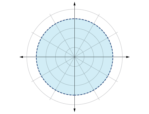
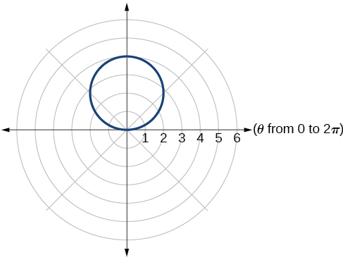
17. circle
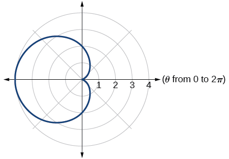
19. cardioid
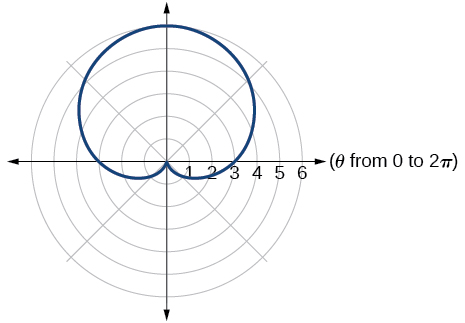
21. cardioid
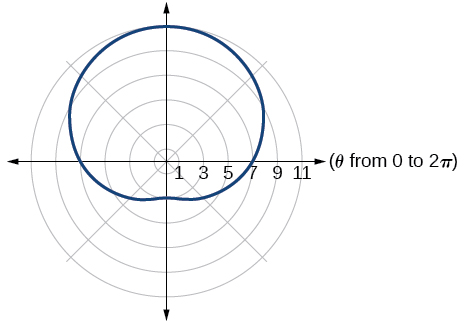
23. one-loop/dimpled limaçon
25. one-loop/dimpled limaçon
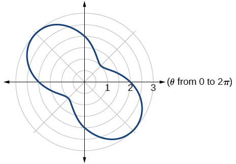
27. inner loop/two-loop limaçon
29. inner loop/two-loop limaçon
31. inner loop/two-loop limaçon
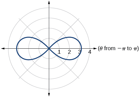
33. lemniscate
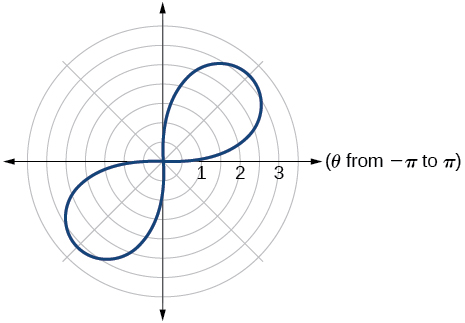
35. lemniscate
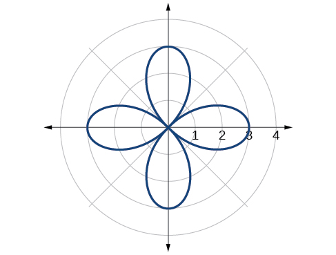
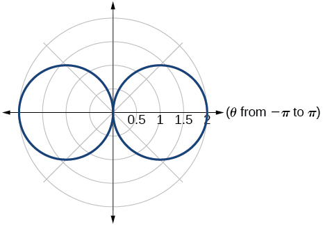
37. rose curve
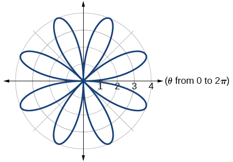
39. rose curve
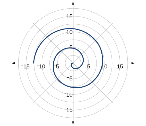
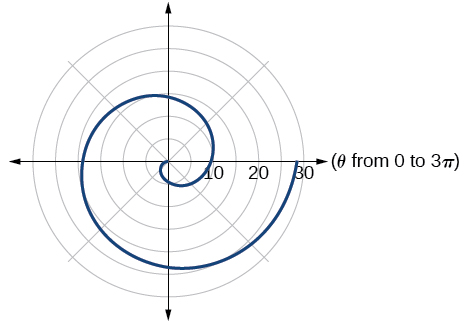
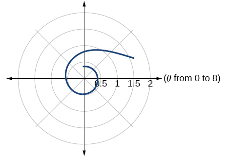
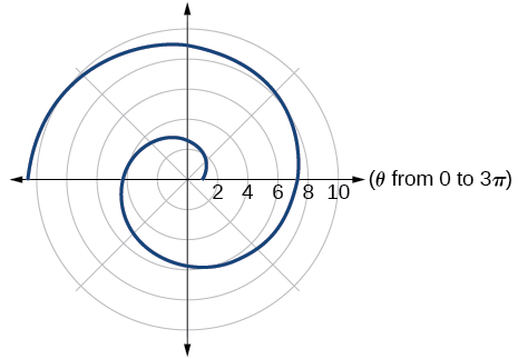
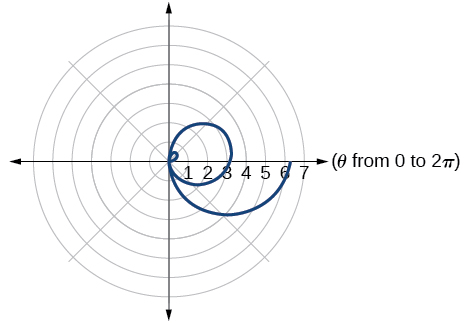
41. Archimedes’ spiral
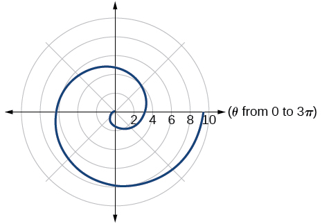
43. Archimedes’ spiral
45.
47.
49.
51.
53.
55. They are both spirals, but not quite the same.
57. Both graphs are curves with 2 loops. The equation with a coefficient of [latex]θ[/latex]
has two loops on the left, the equation with a coefficient of 2 has two loops side by side. Graph these from 0 to [latex]4π[/latex] to get a better picture.
59. When the width of the domain is increased, more petals of the flower are visible.
61. The graphs are three-petal, rose curves. The larger the coefficient, the greater the curve’s distance from the pole.
63. The graphs are spirals. The smaller the coefficient, the tighter the spiral.
65. [latex](4,\frac{π}{3}),(4,\frac{5π}{3})[/latex]
67. [latex](\frac{3}{2},\frac{π}{3}),(\frac{3}{2},\frac{5π}{3})[/latex]
69. [latex](0,\frac{π}{2}), (0,π), (0,3\frac{π}{2}), (0,2π)[/latex]
71. [latex](\frac{\sqrt[4]{8}}{2},\frac{π}{4}), (\frac{\sqrt[4]{8}}{2},\frac{5π}{4})[/latex] and at [latex]θ=\frac{3π}{4}[/latex], [latex]\frac{7π}{4}[/latex] since [latex]r[/latex] is squared
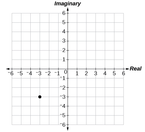
Section 5.5 – Polar Form of Complex Numbers
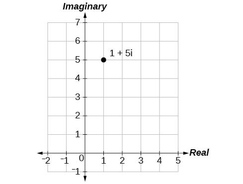
1. a is the real part, b is the imaginary part, and [latex]i=\sqrt{−1}[/latex]
3. Polar form converts the real and imaginary part of the complex number in polar form using [latex]x=rcosθ[/latex] and [latex]y=rsinθ[/latex].
5. [latex]z^n=r^n(cos(nθ)+isin(nθ))[/latex] It is used to simplify polar form when a number has been raised to a power.
7. [latex]5\sqrt{2}[/latex]
9. [latex]\sqrt{38}[/latex]
11. [latex]\sqrt{14.45}[/latex]
13. [latex]4\sqrt{5}cis(333.4∘)[/latex]
15. [latex]2cis(\frac{π}{6})[/latex]
17. [latex]\frac{7\sqrt{3}}{2}+i\frac{7}{2}[/latex]
19. [latex]−2\sqrt{3}−2i[/latex]
21. [latex]−1.5−i\frac{3\sqrt{3}}{2}[/latex]
23. [latex]4\sqrt{3}cis(198∘)[/latex]
25. [latex]\frac{3}{4}cis(180∘)[/latex]
27. [latex]5\sqrt{3}cis(\frac{17π}{24})[/latex]
29. [latex]7cis(70∘)[/latex]
31. [latex]5cis(80∘)[/latex]
33. [latex]5cis(\frac{π}{3})[/latex]
35. [latex]125cis(135∘)[/latex]
37. [latex]9cis(240∘)[/latex]
39. [latex]cis(\frac{3π}{4}[/latex]
41. [latex]3cis(80∘),3cis(200∘),3cis(320∘)[/latex]
43. [latex]2\sqrt[3]{4}cis(\frac{2π}{9}),2\sqrt[3]{4}cis(\frac{8π}{9}),2\sqrt[3]{4}cis(\frac{14π}{9})[/latex]
45. [latex]2\sqrt{2}cis(\frac{7π}{8}),2\sqrt{2}cis(\frac{15π}{8})[/latex]
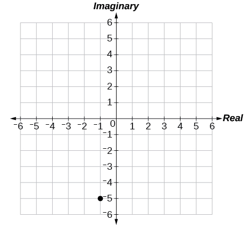
47.
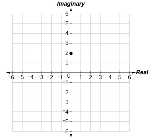
49.
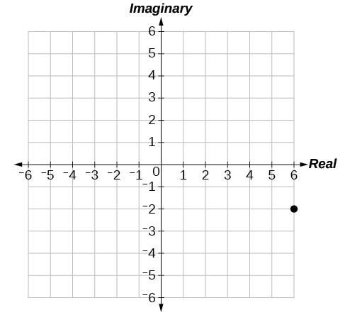
51.
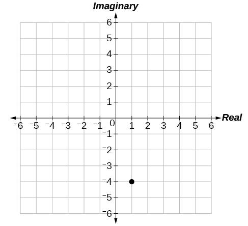
53.
55.
57. [latex]3.61e^{−0.59i}[/latex]
59. [latex]−2+3.46i[/latex]
61. [latex]−4.33−2.50i[/latex]
