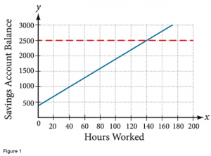
Caroline is a full-time college student planning a spring break vacation. To earn enough money for the trip, she has taken a part-time job at the local bank that pays \$15.00/hr, and she opened a savings account with an initial deposit of \$400 on January 15. She arranged for direct deposit of her payroll checks. If spring break begins March 20 and the trip will cost approximately \$2,500, how many hours will she have to work to earn enough to pay for her vacation? If she can only work 4 hours per day, how many days per week will she have to work? How many weeks will it take? In this section, we will investigate problems like this and others, which generate graphs like the line in Figure 1.

Solving Linear Equations in One Variable

A linear equations is an equation of a straight line, written in one variable. The only power of the variable is 1. Linear equations in one variable may take the form $ax + b = 0$ and are solved using basic algebraic operations.

We begin by classifying linear equations in one variable as one of three types: identity, conditional, or inconsistent. An identity equation is true for all values of the variable. Here is an example of an identity equation.

\[

3x = 2x + x

\]

The solution set consists of all values that make the equation true. For this equation, the solution set is all real numbers because any real number substituted for $x$ will make the equation true.

A conditional equation is true for only some values of the variable. For example, if we are to solve the equation $5x + 2 = 3x – 6$, we have the following:

\begin{align*}

5x + 2 &= 3x – 6 \\

2x &= -8 \\

x &= -4

\end{align*}

The solution set consists of one number: ${-4}$. It is the only solution and, therefore, we have solved a conditional equation.

An inconsistent equation results in a false statement. For example, if we are to solve $5x – 15 = 5(x – 4)$, we have the
following:

\begin{align*}

5x – 15 &= 5(x – 4) \\

5x – 15 &= 5x – 20 \\

5x – 15 – 5x &= -20   &   \text{Subtract $5x$ from both sides.} \\

-15 &\neq -20   &   \text{False statement}

\end{align*}

Indeed, $-15 \neq -20$. There is no solution because this is an inconsistent equation.

Solving linear equations in one variable involves the fundamental properties of equality and basic algebraic operations. A brief review of those operations follows.

How To…

Given a linear equation in one variable, use algebra to solve it.

The following steps are used to manipulate an equation and isolate the unknown variable, so that the last line reads $x = $       , if $x$ is the unknown. There is no set order, as the steps used depend on what is given:

1. We may add, subtract, multiply, or divide an equation by a number or an expression as long as we do the same thing to both sides of the equal sign. Note that we cannot divide by zero.
2. Apply the distributive property as needed: $a(b + c) = ab + ac$.
3. Isolate the variable on one side of the equation.
4. When the variable is multiplied by a coefficient in the final stage, multiply both sides of the equation by the reciprocal of the coefficient.

Finding a Linear Equation

Perhaps the most familiar form of a linear equation is the slope-intercept form, written as $y = mx + b$, where $m =$ slope and $b = y$-intercept. Let us begin with the slope.

The Slope of a Line

The slope of a line refers to the ratio of the vertical change in $y$ over the horizontal change in $x$ between any two points on a line. It indicates the direction in which a line slants as well as its steepness. Slope is sometimes described as rise over run.

\[

m = \dfrac{y_{2} – y_{1}}{x_{2} – x_{1}}

\]

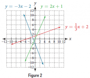
If the slope is positive, the line slants to the right. If the slope is negative, the line slants to the left. As the slope increases, the line becomes steeper. Some examples are shown in Figure 2. The lines indicate the following slopes: $m = -3$, $m = 2$, and $m = \frac{1}{3}$.

The Point-Slope Formula

Given the slope and one point on a line, we can find the equation of the line using the point-slope formula.

\[

y – y_{1} = m(x – x_{1})

\]

This is an important formula, as it will be used in other areas of college algebra and often in calculus to find the equation of a tangent line. We need only one point and the slope of the line to use the formula. After substituting the slope and the coordinates of one point into the formula, we simplify it and write it in slope-intercept form.

Writing and Interpreting an Equation for a Line

Recall that we can write equations in either the slope-intercept form or the point-slope form. Now we can choose which method to use to write equations for a line based on the information we are given. That information may be provided in the form of a graph, a point and a slope, two points, and so on. Look at the graph of the function $f$ in Figure 3.

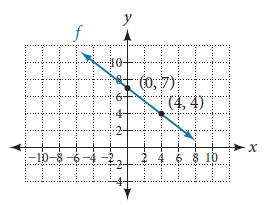
We are not given the slope of the line, but we can choose any two points on the line to find the slope. Let’s choose $(0, 7)$ and $(4, 4)$. We can use these points to calculate the slope.

\begin{align*}

m &= \dfrac{y_{2} – y_{1}}{x_{2} – x_{1}} \\

&= \dfrac{4 – 7}{4 – 0} \\

&= -\dfrac{3}{4}

\end{align*}

Now we can substitute the slope and the coordinates of one of the points into the point-slope form.

\begin{align*}

y – y_{1} &= m(x – x_{1}) \\

y – 4 &= -\dfrac{3}{4} (x – 4)

\end{align*}

If we want to rewrite the equation in the slope-intercept form, we would find

\begin{align*}

y – 4 &= -\dfrac{3}{4} (x – 4) \\

y – 4 &= -\dfrac{3}{4}x + 3 \\

y &= -\dfrac{3}{4}x + 7

\end{align*}

If we wanted to find the slope-intercept form without first writing the point-slope form, we could have recognized that the line crosses the $y$-axis when the output value is 7. Therefore, $b = 7$. We now have the initial value $b$ and the slope $m$ so we can substitute $m$ and $b$ into the slope-intercept form of a line.

\[

y = mx + b

\]

How To…

Given the graph of a linear equation, write an equation to represent the equation.

1. Identify two points on the line.
2. Use the two points to calculate the slope.
3. Determine where the line crosses the $y$-axis to identify the $y$-intercept by visual inspection.
4. Substitute the slope and $y$-intercept into the slope-intercept form of a line equation.

Example 7  Writing an Equation for a Line

Write an equation for a line given a graph of $f$ shown in Figure 4.

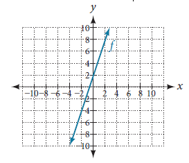
Solution  Identify two points on the line, such as $(0, 2)$ and $(-2, -4)$. Use the points to calculate the slope.

\begin{align*}

m &= \dfrac{y_{2} – y_{1}}{x_{2} – x_{1}} \\

&= \dfrac{-4 – 2}{-2 – 0} \\

&= \dfrac{-6}{-2} \\

&= 3

\end{align*}

Substitute the slope and the coordinates of one of the points into the point-slope form.

\begin{align*}

y – y_{1} &= m (x – x_{1}) \\

y – (-4) &= 3(x – (-2)) \\

y + 4 &= 3(x + 2) \\

y + 4 &= 3x + 6 \\

y &= 3x + 2

\end{align*}

Graphing Linear Equations

Now that we’ve seen and interpreted graphs of lines, let’s take a look at how to create the graphs. There are three basic methods of graphing lines. The first is by plotting points and then drawing a line through the points. The second is by using the $y$-intercept and slope. And the third method is by using transformations of the identity function $f(x) = x$.

Graphing a Line by Plotting Points

To find points of a line, we can choose input values, evaluate the function at these input values, and calculate output values. The input values and corresponding output values form coordinate pairs. We then plot the coordinate pairs on a grid. In general, we should evaluate the function at a minimum of two inputs in order to find at least two points on the graph. For example, given the function, $f(x) = 2x$, we might use the input values 1 and 2. Evaluating the function for an input value of 1 yields an output value of 2, which is represented by the point $(1, 2)$. Evaluating the function for an input value of 2 yields an output value of 4, which is represented by the point $(2, 4)$. Choosing three points is often advisable because if all three points do not fall on the same line, we know we made an error.

How To…

Given a line, graph by plotting points.

1. Choose a minimum of two input values.
2. Evaluate the function at each input value.
3. Use the resulting output values to identify coordinate pairs.
4. Plot the coordinate pairs on a grid.
5. Draw a line through the points.

Example 8  Graphing by Plotting Points

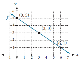
Graph $f(x) = -\frac{2}{3}x + 5$ by plotting points.

Solution  Begin by choosing input values. This function includes a fraction with a denominator of 3, so let’s choose multiples of 3 as input values. We will choose 0, 3, and 6.

Evaluate the function at each input value, and use the output value to identify coordinate pairs.

$x$-value	$y$-value	Point
$x = 0$	$y = -\frac{2}{3}(0) + 5 = 5$	$(0, 5)$
$x = 3$	$y = -\frac{2}{3}(3) + 5 = 3$	$(3, 3)$
$x = 6$	$y = -\frac{2}{3}(6) + 5 = 1$	$(6, 1)$

Plot the coordinate pairs and draw a line through the points. Figure 5 represents the graph of the line $y = -\frac{2}{3}x + 5$.

Graphing a Line Using y-intercept and Slope

Another way to graph a line is by using specific characteristics rather than plotting points. The first characteristic is its $y$-intercept, which is the point at which the input value is zero. To find the $y$-intercept, we can set $x = 0$ in the equation.

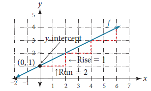
The other characteristic of the line is its slope. Let’s consider the linear equation $y = \frac{1}{2}x + 1$. The slope is $\frac{1}{2}$. Because the slope is positive, we know the graph will slant upward from left to right. The $y$-intercept is the point on the graph when $x = 0$. The graph crosses the $y$-axis at $(0, 1)$. Now we know the slope and the $y$-intercept. We can begin graphing by plotting the point $(0, 1)$. We know that the slope is rise over run, $m = \dfrac{\text{rise}}{\text{run}}$. From our example, we have $\frac{1}{2}$, which means that the rise is 1 and the run is 2. So starting from our $y$-intercept $(0, 1)$, we can rise 1 and then run 2, or run 2 and then rise 1. We repeat until we have a few points, and then we draw a line through the points as shown in Figure 6.