19 Exponential Functions
Topics Covered:
Define and Evaluate Exponential Functions[1]
India is the second most populous country in the world with a population of about 1.39 billion people in 2021. The population is growing at a rate of about 1.2% each year [2] If this rate continues, the population of India will exceed China’s population by the year 2027. When populations grow rapidly, we often say that the growth is “exponential,” meaning that something is growing very rapidly. To a mathematician, however, the term exponential growth has a very specific meaning. In this section, we will take a look at exponential functions, which model this kind of rapid growth.
When exploring linear equations, we observed a constant rate of change—a constant number by which the output increased for each unit increase in input. For example, in the equation  , the slope tells us the output increases by 3 each time the input increases by 1. The scenario in the India population example is different because we have a percent change per unit of time (rather than a constant change) in the number of people.
What exactly does it mean to grow exponentially? What does the word double have in common with the percent increase?
- Percent change refers to a change based on a percent of the original amount.
- Exponential growth refers to an increase based on a constant multiplicative rate of change over equal increments of time, that is, a percent increase of the original amount over time.
- Exponential decay refers to a decrease based on a constant multiplicative rate of change over equal increments of time, that is, a percent decrease of the original amount over time.
For us to gain a clear understanding of exponential growth, let us contrast exponential growth with linear growth. We will construct two functions. The first function is exponential. We will start with an input of 0, and increase each input by 1. We will double the corresponding consecutive outputs. The second function is linear. We will start with an input of 0, and increase each input by 1. We will add 2 to the corresponding consecutive outputs. See the table below
 |
 |
 |
|---|---|---|
| 0 | 1 | 0 |
| 1 | 2 | 2 |
| 2 | 4 | 4 |
| 3 | 8 | 6 |
| 4 | 16 | 8 |
| 5 | 10 | 32 |
| 6 | 64 | 12 |
From the table we can infer that for these two functions, exponential growth dwarfs linear growth.
- Exponential growth refers to the original value from the range increasing by the same percentage over equal increments found in the domain.
- Linear growth refers to the original value from the range increasing by the same amount over equal increments found in the domain.
Apparently, the difference between “the same percentage” and “the same amount” is quite significant. For exponential growth, over equal increments, the constant multiplicative rate of change resulted in doubling the output whenever the input increased by one. For linear growth, the constant additive rate of change over equal increments resulted in adding 2 to the output whenever the input was increased by one.
While we explore more about the growth and decay in the next section, we will first look at the equation for exponential functions. The general form of the exponential function is  , where a is any nonzero number, b is a positive real number not equal to 1.
For any real number  , an exponential function is a function with the form:

where,
- a is a non-zero real number called the initial value
- b is any positive real number (b >0), such that b ≠ 1
- Note you may also see the function as
 , and where b >0 and b ≠ 1.
Notice that in this function, the variable is the exponent. In our functions so far, the variables were the base.
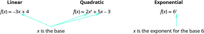
Recall that the base of an exponential function must be a positive real number other than 1. Why do we limit the base b to positive values? To ensure that the outputs will be real numbers. Observe what happens if the base is not positive:


 not a real number
In fact, f(x) = (−4)xwould not be a real number any time x is a fraction with an even denominator. So our definition requires b > 0.
Try it! – Identifying Exponential Functions
- Which of the following equations are not exponential functions?


Solution
By definition, an exponential function has a constant as a base and an independent variable as an exponent. Thus, g(x) = x3 does not represent an exponential function because the base is an independent variable. In fact, g(x) = x3is a power function.
Recall that the base a of an exponential function is always a positive constant, and b ≠ 1. Thus, j(x) = (−2)x does not represent an exponential function because the base, −2, is less than 0.
2. Which of the following equations represent exponential functions?
- f(x) = 2x2 − 3x + 1
- g(x) = 0.875x
- h(x) = 1.75x + 2
- j(x) = 1095.6-2x
Solution
g(x) = 0.875xand j(x) = 1095.6-2x represent exponential functions.
Why do we limit the base to positive values other than 1? Because base 1 results in the constant function. Observe what happens if the base is 1:
- Let b = 1. Then f(x) = 1x = 1 for any value of x.
To evaluate an exponential function with the form f(x) =a(b)x, we simply substitute x with the given value, and calculate the resulting power. For example:
Let f(x) = 2x. What is f(3)?
To evaluate an exponential function with a form other than the basic form, it is important to follow the order of operations. For example:
Let f(x) =30(2)x . What is f(3)?
Note that if the order of operations were not followed, the result would be incorrect:
Try it! – Evaluating Exponential Functions
- Let f(x) = 5(3)x + 1. Evaluate f(2) without using a calculator.
Solution
Follow the order of operations. Be sure to pay attention to the parentheses.
2. Let f(x) = 8(1.2)x – 5. Evaluate f(3) using a calculator. Round to four decimal places.
Solution
5.5556
Exponential Growth and Decay [3]
The term “exponential growth” is often used in everyday language to describe anything that grows or increases rapidly. However, exponential growth can be defined more precisely in a mathematical sense. If the growth rate is proportional to the amount present, the function models exponential growth.
Exponential growth grows by a rate proportional to the amount present.
The exponential functions grow faster the larger the input value is. This means that the larger the amount, the faster it will grow. AND not only will the amount itself grow larger, but the rate at which it grows will also increase.
For any real number x and any positive real numbers a and b such that b ≠ 1, an exponential growth function has the form where
- a is the initial or starting value of the function.
- b is the growth factor or growth multiplier per unit x . Also called the base.
In more general terms, we have an exponential function, in which a constant base is raised to a variable exponent. To differentiate between linear and exponential functions in a more practical example, let’s consider two companies, A and B. Company A has 100 stores and expands by opening 50 new stores a year, so its growth can be represented by the function  . Company B has 100 stores and expands by increasing the number of stores by 50% each year, so its growth can be represented by the function
  . Notice the distinction we mentioned earlier. Company A changes by the same amount per year (50 stores opened each year), while Company B exhibits a percent increase each year (# of stores increases by 50% per year). So again we are seeing a percentage change rather than a constant change. A few years of growth for these companies are illustrated below:
| Year, x | Stores, Company A | Stores, Company B |
| 0 |  |
 |
| 1 |  |
 |
| 2 |  |
 |
| 3 |  |
 |
| x | |
 |
We can see in the graphs that, with exponential growth, the number of stores increases much more rapidly than with linear growth.
Notice that the domain (all of the x-values) for both functions is  , and the range (all of the y-values) for both functions is
  . After year 1, Company B always has more stores than Company A.
Now we will turn our attention to the function representing the number of stores for Company B,  . In this exponential function, 100 represents the initial number of stores, 0.50 represents the growth rate, and
  represents the growth factor. Generalizing further, we can write this function as
  , where 100 is the initial value, 1.5 is called the base, and x is called the exponent.
A note of caution if you are working with growth rate vs growth factor. In this example it specifies the expansion increases by (a rate of) 50% annually, this is growth rate (r). To determine the growth factor (our b value), use (1 + r) if the amount is increasing and if it is decreasing the decay factor (still our b value) use (1 – r). In the example, the growth factor (b in our equation) is 1+0.5. Also keep in mind that r is often given as a percentage, which should always be converted to decimal form before it is plugged into the equation.
Try it! – Evaluating a Real-World Exponential Model
At the beginning of this section, we learned that the population of India was about 1.25 billion in the year 2013, with an annual growth rate of about 1.2%. This situation is represented by the growth function  , where t is the number of years since 2013. To the nearest thousandth, what will the population of India be in 2031?
Solution
To estimate the population in 2031, we evaluate the models for t=18, because 2031 is 18 years after 2013. Rounding to the nearest thousandth,

There will be about 1.549 billion people in India in the year 2031.
Try it! Writing an Exponential Model When the Initial Value Is Known
In 2006, 80 deer were introduced into a wildlife refuge. By 2012, the population had grown to 180 deer. The population was growing exponentially. Write an exponential function  representing the population (N) of deer over time t.
Solution
We let our independent variable t be the number of years after 2006. Thus, the information given in the problem can be written as input-output pairs: (0, 80) and (6, 180). Notice that by choosing our input variable to be measured as years after 2006, we have given ourselves the initial value for the function,  . We can now substitute the second point into the equation
  to find b:
| Steps | Algebraic |
|---|---|
 |
|
| Substitute using point (6, 180). |  |
| Divide and write in lowest terms. |  |
| Isolate busing properties of exponents. |  |
| Round to 4 decimal places. |  |
NOTE: Unless otherwise stated, do not round any intermediate calculations. Then round the final answer to four places for the remainder of this section.
The exponential model for the population of deer is  . (Note that this exponential function models short-term growth. As the inputs gets large, the output will get increasingly larger, so much so that the model may not be useful in the long term.)
We can graph our model to observe the population growth of deer in the refuge over time. Notice that the graph in the image below passes through the initial points given in the problem, (0,80) and (6,180). We can also see that the domain for the function is , and the range for the function is  .
.
In these examples our function has been dealing with an increase or growth. But what if it is the opposite, decreasing, or what is called decay. Let’s try an example similar to the population example above, just with a decreasing population.
Try it!
In 2006, 200 deer were introduced into a wildlife refuge. By 2012, the population had dropped to 125 deer. The population was decreasing exponentially. Write an exponential function representing the population  of deer over time t.
Solution
To estimate the population in 2031, we evaluate the models for t = 6 , because 2012 is 6 years after 2006. Our a value is the initial population in 2006, 200 deer.


The exponential model for the population of deer is  .
.
In the exponential function modeling growth of the form we can also use the following rules to help identify if something is growth, decay, or neither
- If b > 1, it is growth
- If 0 < b > 1, it is decay
Try it!
#1
We have the equation  the base (growth factor) is 1.25. Following our rules, we want to identify if b is greater than 1 or is between 0 and 1.
Solution
As 1.25 is greater than 1, it would represent growth.
#2
We have the equation  . what is our b value? Is it growing or decaying?
Solution
b is 0.58. As this is between 0 and 1, it would be decreasing or decay.
#3
For the following exercises, determine whether the equation represents exponential growth, exponential decay, or neither. Explain.
a. 
b. 
c. 
d. 
Solution
a. exponential growth; The growth factor, 1.06, is greater than 1.
b. exponential decay; The decay factor, 0.97, is between 0 and 1.
c. exponential decay; The decay factor, 0.825, is between 0 and 1.
d. neither. The base value b is negative, meaning that it is not exponential.
Graphing Exponential Functions
By graphing a few exponential functions, we will be able to see their unique properties. In the cases below, we will use the form of f(x) = bx for exponential functions.
Try it!
- On the same coordinate system graph f(x) = 2x and g(x) = 3x.
Solution
We will use point plotting to graph the functions.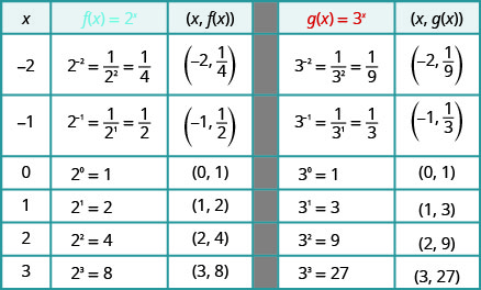
2. Graph: g(x) = 5x.
Solution
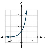
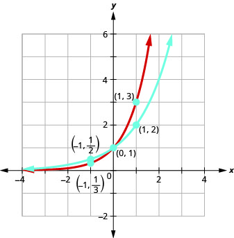
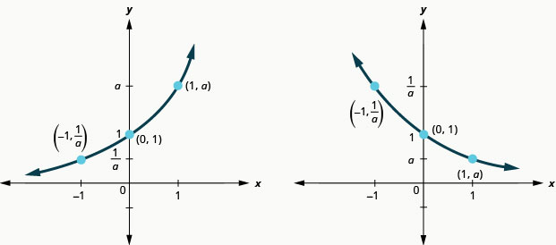
The graphs of f(x) = 2x and g(x) = 3x, as well as the graphs of f(x) = 4x and g(x) = 5x, all have the same basic shape. This is the shape we expect from an exponential function where a > 1.
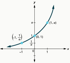
We notice, that for each function, the graph contains the point (0, 1). This make sense because a0 = 1 for any a.
The graph of each function, f(x) = ax also contains the point (1, a). The graph of f(x) = 2x contained (1, 2) and the graph of g(x) = 3x contained (1, 3). This makes sense as a1 = a.
Notice too, the graph of each function f(x) = ax also contains the point  . The graph of f(x) = 2x contained
  and the graph of g(x) = 3x contained
  . This makes sense as
  .
.
What is the domain for each function? From the graphs we can see that the domain is the set of all real numbers. There is no restriction on the domain. We write the domain in interval notation as (−∞, ∞).
Look at each graph. What is the range of the function? The graph never hits the x-axis. The range is all positive numbers. We write the range in interval notation as (0, ∞).
Whenever a graph of a function approaches a line but never touches it, we call that line an asymptote. For the exponential functions we are looking at, the graph approaches the x-axis very closely but will never cross it, we call the line y = 0, the x-axis, a horizontal asymptote.
Properties of the Graph of f(x) = ax when a > 1
| Properties | Definition |
| Domain | (−∞, ∞) |
| Range | (0, ∞) |
| x–intercept | None |
| y–intercept | (0, 1) |
| Contains | (1, a),  |
| Asymptote |
x-axis, the line y = 0 |
Our definition of an exponential function f(x) = ax says a > 0, but the examples and discussion so far has been about functions where a > 1. What happens when 0 < a < 1? The next example will explore this possibility.
Try it!
- On the same coordinate system, graph
 and
and  .
.
Solution
We will use point plotting to graph the functions.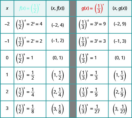
2. Graph:  .
.
Solution
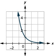
3. Graph:  .
.
Solution
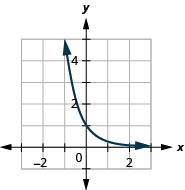
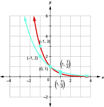
Now let’s look at the graphs from the previous Example and Try Its so we can now identify some of the properties of exponential functions where 0 < a < 1.
The graphs of and as well as the graphs of and all have the same basic shape. While this is the shape we expect from an exponential function where 0 < a < 1, the graphs go down from left to right while the previous graphs, when a > 1, went from up from left to right.
We notice that for each function, the graph still contains the point (0, 1). This makes sense because a0 = 1 for any a.
As before, the graph of each function, f(x) = ax, also contains the point (1, a). The graph of contained  and the graph of contained
  . This makes sense as a1 = a.
Notice too that the graph of each function, f(x) = ax, also contains the point . The graph of contained (−1, 2) and the graph of contained (−1, 3). This makes sense as .
We will summarize these properties in the chart below. Which also include when a > 1.
Properties of the Graph of f(x) = ax
| when a > 1 | when 0 < a < 1 | ||
|---|---|---|---|
| Domain | (−∞, ∞) | Domain | (−∞, ∞) |
| Range | (0, ∞) | Range | (0, ∞) |
| x-intercept | none | x-intercept | none |
| y-intercept | (0, 1) | y-intercept | (0,1 ) |
| Contains | (1, a), |
Contains | (1, a), |
| Asymptote | x-axis, the line y = 0 | Asymptote | x-axis, the line y = 0 |
| Basic shape | increasing | Basic shape | decreasing |
It is important for us to notice that both of these graphs are one-to-one, as they both pass the horizontal line test. This means the exponential function will have an inverse. We will look at this later.
Natural Base e
All of our exponential functions have had either an integer or a rational number as the base. We will now look at an exponential function with an irrational number as the base.
Before we can look at this exponential function, we need to define the irrational number, e. This number is used as a base in many applications in the sciences and business that are modeled by exponential functions. The number is defined as the value of  as n gets larger and larger. We say, as n approaches infinity, or increases without bound. The table shows the value of for several values of n.
| n | |
|---|---|
| 1 | 2 |
| 2 | 2.25 |
| 5 | 2.48832 |
| 10 | 2.59374246 |
| 100 | 2.704813829… |
| 1,000 | 2.716923932… |
| 10,000 | 2.718145927… |
| 100,000 | 2.718268237… |
| 1,000,000 | 2.718280469… |
| 1,000,000,000 | 2.718281827… |
The number e is like the number π in that we use a symbol to represent it because its decimal representation never stops or repeats. The irrational number e is called the natural base.
Natural Base e
The number e is defined as the value of , as n increases without bound. We say, as n approaches infinity,
e ≈ 2.718281827…
The exponential function whose base is e, f(x) = ex is called the natural exponential function.
Natural Exponential Function
The natural exponential function is an exponential function whose base is e:
f(x) = ex
The domain is (−∞, ∞) and the range is (0, ∞).
Let’s graph the function f(x) = ex on the same coordinate system as g(x) = 2x and h(x) = 3x.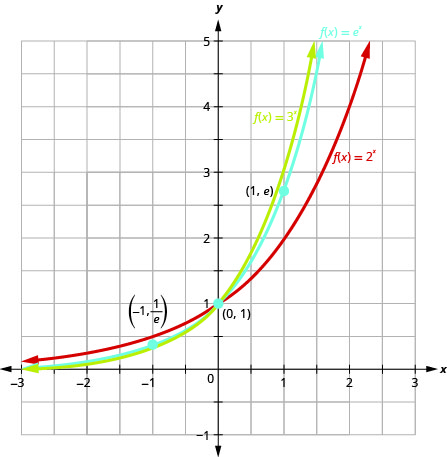 Notice that the graph of f(x) = ex is “between” the graphs of g(x) = 2x and h(x) = 3x. Does this make sense as 2 < e < 3?
Use Exponential Models in Applications
Exponential functions model many situations. If you own a bank account, you have experienced the use of an exponential function. There are two formulas that are used to determine the balance in the account when interest is earned. If a principal, P, is invested at an interest rate, r, for t years, the new balance, A, will depend on how often the interest is compounded. If the interest is compounded n times a year we use the formula  . If the interest is compounded continuously, we use the formula A = Pert. These are the formulas for compound interest.
Compound Interest
For a principal, P, invested at an interest rate, r, for t years, the new balance, A, is:
when compounded n times a year.
A = Pert when compounded continuously.
As you work with the Interest formulas, it is often helpful to identify the values of the variables first and then substitute them into the formula.
Try it!
- A total of $10,000 was invested in a college fund for a new grandchild. If the interest rate is 5%,how much will be in the account in 18 years by each method of compounding?
a. compound quarterly
b. compound monthly
c. compound continuously
Solution
| Steps | Algebraic |
| A = ? | |
| Identify the values of each variable in the formulas. | P = $10,000 |
| Remember to express the percent as a decimal. | r = 0.05 |
| t = 18 years |
a.
| Steps | Algebraic |
| For quarterly compounding, n = 4. There are 4 quarters in a year. | |
| Substitute the values in the formula |  |
| Compute the amount. Be careful to consider the order of operations as you enter the expression into your calculator. | A = $24,459.20 |
b.
| Steps | Algebraic |
| For monthly compounding, n = 12. There are 12 months in a year. | |
| Substitute the values in the formula. |  |
| Compute the amount. | A = $24,550.08 |
c.
| Steps | Algebraic |
| For compounding continuously, | A = Pert |
| Substitute the values in the formula. |  |
| Compute the amount. | A = $24,596.03 |
2. Angela invested $15,000 in a savings account. If the interest rate is 4%, how much will be in the account in 10 years by each method of compounding?
a. compound quarterly
b. compound monthly
c. compound continuously
Solution
a. $22,332.96
b. $22,362.49
c. $22,377.37
Access these online resources for additional instruction and practice with evaluating and graphing exponential functions.
Key Concepts
- Properties of the Graph of f(x) = ax
when a > 1 when 0 < a < 1 Domain (−∞, ∞) Domain (−∞, ∞) Range (0, ∞) Range (0, ∞) x-intercept none x-intercept none y-intercept (0, 1) y-intercept (0, 1) Contains (1, a), Contains (1, a), Asymptote x-axis, the line y = 0 Asymptote x-axis, the line y = 0 Basic shape increasing Basic shape decreasing 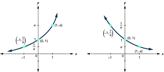 Compound Interest: For a principal, P, invested at an interest rate, r, for t years, the new balance, A, is
- when compounded n times a year.
- A = Pert when compounded continuously.
- Section material derived from Openstax College Algebra: Exponential and Logarithmic Functions-Exponential Functions and Intermediate Algebra: Exponential and Logarithmic Functions-Evaluate and Graph Exponential Functions ↵
- http://www.worldometers.info/world-population/. Accessed February 24, 2014. ↵
- Section material derived from Openstax College Algebra: Exponential and Logarithmic Functions-Exponential Functions ↵
is a function of the form f(x) = a^x where a > 0 and a ≠ 1.
A rate of growth that increases in proportion to the original population
A line which a graph of a function approaches closely but never touches.
The number e is defined as the value of (1+ [latex]\displaystyle \frac{1}{n}[/latex])n, as n increases without bound. We say, as n approaches infinity, e ≈ 2.718281827..
The natural exponential function is an exponential function whose base is e: f(x) = ex
The domain is (−∞,∞) and the range is (0,∞).
