8 Measuring the Spread of Data
Topics Covered:[1]
In case you missed something in class, or just want to review a specific topic covered in this Module, here is a list of topics covered:
Data Sampling
In statistics, we generally want to study a population. You can think of a population as a collection of persons, things, or objects under study. Gathering information about an entire population often costs too much or is virtually impossible. Instead, we use a sample of the population. A sample should have the same characteristics as the population it is representing. The idea of sampling is to select a portion (or subset) of the larger population and study that portion (the sample) to gain information about the population. Data are the result of sampling from a population.
Most statisticians use various methods of random sampling in an attempt to achieve this goal.
Random Sample
A random sample is a representative group from the population chosen by using a method that gives each individual in the population an equal chance of being included in the sample.
There are several different methods of random sampling. The easiest method to describe is called a simple random sample. Any group of n individuals is equally likely to be chosen as any other group of n individuals if the simple random sampling technique is used. In other words, each sample of the same size has an equal chance of being selected.
If we were to examine two samples representing the same population, even if we used random sampling methods for the samples, they would not be exactly the same. Just as there is variation in data, there is variation in samples. As you become accustomed to sampling, the variability will begin to seem natural.
Samples that contain different individuals result in different data. This is true even when the samples are well-chosen and representative of the population. When properly selected, larger samples model the population more closely than smaller samples. There are many different potential problems that can affect the reliability of a sample. Statistical data needs to be critically analyzed, not simply accepted.
From the sample data, we can calculate a statistic. A statistic is a number that represents a property of the sample. For example, if we consider one math class to be a sample of the population of all math classes, then the average number of points earned by students in that one math class at the end of the term is an example of a statistic. The statistic is an estimate of a population parameter. A parameter is a numerical characteristic of the whole population that can be estimated by a statistic. Since we considered all math classes to be the population, then the average number of points earned per student over all the math classes is an example of a parameter.
Try it!
Determine what the key terms refer to in the following study. We want to know the average (mean) amount of money first year college students spend at ABC College on school supplies that do not include books. We randomly surveyed 100 first year students at the college. Three of those students spent $150, $200, and $225, respectively.
Solution (click to reveal)
The population is all first-year students attending ABC College this term.
The sample could be all students enrolled in one section of a beginning statistics course at ABC College (although this sample may not represent the entire population).
The parameter is the average (mean) amount of money spent (excluding books) by first year college students at ABC College this term.
The statistic is the average (mean) amount of money spent (excluding books) by first year college students in the sample.
The variable could be the amount of money spent (excluding books) by one first year student. Let X = the amount of money spent (excluding books) by one first year student attending ABC College.
The data are the dollar amounts spent by the first year students. Examples of the data are $150, $200, and $225.
Determine what the key terms refer to in the following study.
A study was conducted at a local college to analyze the average cumulative GPAs of students who graduated last year. Fill in the letter of the phrase that best describes each of the items below.
1. Population_ 2. Statistic _ 3. Parameter _ 4. Sample _ 5. Variable _ 6. Data _
- all students who attended the college last year
- the cumulative GPA of one student who graduated from the college last year
- 3.65, 2.80, 1.50, 3.90
- a group of students who graduated from the college last year, randomly selected
- the average cumulative GPA of students who graduated from the college last year
- all students who graduated from the college last year
- the average cumulative GPA of students in the study who graduated from the college last year
Solution (click to reveal)
- f;
- g;
- e;
- d;
- b;
- c
The Central Limit Theorem
Remember, from Measures of Central Tendencies, the mean of a set of data is the result of dividing the sum of the values by the number of values.
There are two types of means that we will analyze: the sample mean and the population mean.
As is implied by their names, the population mean is the mean of the population being investigated. The sample mean is the mean of the sample taken from the population being investigated.
The letter used to represent the sample mean is an x with a bar over it (pronounced “x bar”):

The Greek letter  (pronounced “mew”) represents the population mean.
One of the requirements for the sample mean to be a good estimate of the population mean is for the sample taken to be truly random.
The central limit theorem for sample means says that if you keep drawing larger and larger samples (such as rolling one, two, five, and finally, ten dice) and calculating their means, the sample means form their own normal distribution (the sampling distribution). As sample sizes increase, the distribution of means more closely follows the normal distribution. The normal distribution has the same mean as the original distribution and a variance that equals the original variance divided by the sample size. Standard deviation is the square root of variance, so the standard deviation of the sampling distribution is the standard deviation of the original distribution divided by the square root of n. The variable n is the number of values that are averaged together, not the number of times the experiment is done.
To put it more formally, if you draw random samples of size n, the distribution of the random variable  , which consists of sample means, is called the sampling distribution of the mean. The sampling distribution of the mean approaches a normal distribution as n, the sample size, increases.
The Law of Large Numbers says that if you take samples of larger and larger size from any population, then the mean  of the sample is very likely to get closer and closer to
  . From the central limit theorem, we know that as n gets larger and larger, the sample means follow a normal distribution. The larger n gets, the smaller the standard deviation gets. We can say that is the value that the sample means approach as n gets larger. The central limit theorem illustrates the law of large numbers.
The Standard Deviation
An important characteristic of any set of data is the variation in the data. In some data sets, the data values are concentrated closely near the mean; in other data sets, the data values are more widely spread out from the mean. The most common measure of variation, or spread, is the standard deviation.
The standard deviation is a number that measures how far data values are from their mean.
- provides a numerical measure of the overall amount of variation in a data set.
- shows how spread out the data are about the mean.
- is always positive or zero.
- is small when the data are all concentrated close to the mean, exhibiting little variation or spread and is larger when the data values are more spread out from the mean, exhibiting more variation.
- a positive deviation occurs when the data value is greater than the mean, whereas a negative deviation occurs when the data value is less than the mean.
- can be used to determine whether a particular data value is close to or far from the mean.
- If you add the deviations, the sum is always zero. So you cannot simply add the deviations to get the spread of the data.
If x is a number, then the difference “x – mean” is called its deviation. In a data set, there are as many deviations as there are items in the data set. The deviations are used to calculate the standard deviation. If the numbers belong to a population, in symbols a deviation is  . For sample data, in symbols a deviation is
  .
.
The lower case letter s represents the sample standard deviation and the Greek letter  (sigma, lower case) represents the population standard deviation. If the sample has the same characteristics as the population, then s should be a good estimate of .
To calculate the standard deviation, we need to calculate the variance first. The variance is the average of the squares of the deviations (the ) values for a sample, or the values for a population). The symbol  represents the population variance; the population standard deviation is the square root of the population variance. The symbol s2 represents the sample variance; the sample standard deviation s is the square root of the sample variance. You can think of the standard deviation as a special average of the deviations.
If the numbers come from a census of the entire population and not a sample, when we calculate the average of the squared deviations to find the variance, we divide by N, the number of items in the population. If the data are from a sample rather than a population, when we calculate the average of the squared deviations, we divide by n – 1, one less than the number of items in the sample.
Formulas for the Sample & Population Standard Deviation
Sample standard deviation:

For the sample standard deviation, the denominator is n – 1, that is the sample size MINUS 1.
Population standard deviation:

For the population standard deviation, the denominator is N, the number of items in the population.
Your concentration should be on what the standard deviation tells us about the data. The standard deviation is a number which measures how far the data are spread from the mean. Let a calculator or computer do the arithmetic.
The standard deviation,  , is either zero or larger than zero. Describing the data with reference to the spread is called “variability”. The variability in data depends upon the method by which the outcomes are obtained; for example, by measuring or by random sampling. When the standard deviation is zero, there is no spread; that is, the all the data values are equal to each other. The standard deviation is small when the data are all concentrated close to the mean, and is larger when the data values show more variation from the mean. When the standard deviation is a lot larger than zero, the data values are very spread out about the mean; outliers can make s or very large.
The standard deviation, when first presented, can seem unclear. By graphing your data, you can get a better “feel” for the deviations and the standard deviation. You will find that in symmetrical distributions, the standard deviation can be very helpful but in skewed distributions, the standard deviation may not be much help. The reason is that the two sides of a skewed distribution have different spreads. In a skewed distribution, it is better to look at the first quartile, the median, the third quartile, the smallest value, and the largest value. Because numbers can be confusing, always graph your data. Display your data in a histogram or a box plot.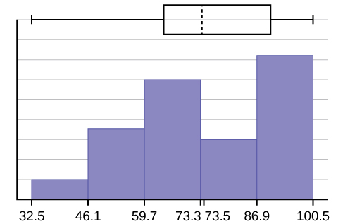
The following lists give a few facts that provide a little more insight into what the standard deviation tells us about the distribution of the data.
- At least 75% of the data is within two standard deviations of the mean.
- At least 89% of the data is within three standard deviations of the mean.
- At least 95% of the data is within 4.5 standard deviations of the mean.
- Approximately 68% of the data is within one standard deviation of the mean.
- Approximately 95% of the data is within two standard deviations of the mean.
- More than 99% of the data is within three standard deviations of the mean.
- This is known as the Empirical Rule.
It is important to note that this rule only applies when the shape of the distribution of the data is bell-shaped and symmetric. We will learn more about this when studying the “Normal” or “Gaussian” probability distribution in later chapters.
The Normal Distribution
The normal, a continuous distribution, is the most important of all the distributions. It is widely used and even more widely abused. Its graph is bell-shaped. You see the bell curve in almost all disciplines. Some of these include psychology, business, economics, the sciences, nursing, and, of course, mathematics. Some of your instructors may use the normal distribution to help determine your grade. Most IQ scores are normally distributed. Often real-estate prices fit a normal distribution. The normal distribution is extremely important, but it cannot be applied to everything in the real world.
The normal distribution has two parameters (two numerical descriptive measures): the mean (μ) and the standard deviation (σ). We can say that X is a quantity to be measured that has a normal distribution with mean (μ) and standard deviation (σ).
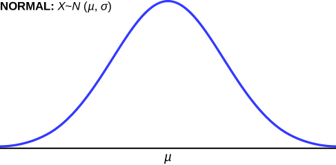
The curve is symmetric about a vertical line drawn through the mean, . In theory, the mean is the same as the median, because the graph is symmetric about . As the notation indicates, the normal distribution depends only on the mean and the standard deviation. Since the area under the curve must equal one, a change in the standard deviation, , causes a change in the shape of the curve; the curve becomes fatter or skinnier depending on . A change in causes the graph to shift to the left or right. This means there are an infinite number of normal probability distributions.
For a normally distributed set of data that follows this normal curve, some important facts about the spread of the data can be stated:
Empirical Rule:
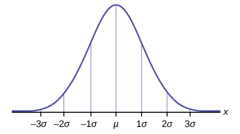
If X is a random variable and has a normal distribution with mean and standard deviation , then the Empirical Rule states the following:
- About 68% of the x values lie between –1 and +1 of the mean (within one standard deviation of the mean).
- About 95% of the x values lie between –2 and +2 of the mean (within two standard deviations of the mean).
- About 99.7% of the x values lie between –3 and +3 of the mean (within three standard deviations of the mean). Notice that almost all the x values lie within three standard deviations of the mean.
This allows for the normal curve to be split into quadrants or groups of data as is shown below. Where is the population mean, and is the standard deviation of the data.
Key Concepts
-
-
- Standard Deviation
- Sample standard deviation:Population standard deviation:
- Sample standard deviation:
- Empirical Rule: If X is a random variable and has a normal distribution with mean µ and standard deviation σ, then the Empirical Rule states the following:
- About 68% of the x values lie between –1 and +1 of the mean (within one standard deviation of the mean).
- About 95% of the x values lie between –2 and +2 of the mean (within two standard deviations of the mean).
- About 99.7% of the x values lie between –3 and +3 of the mean (within three standard deviations of the mean). Notice that almost all the x values lie within three standard deviations of the mean.
- About 68% of the x values lie between –1
- Standard Deviation
-
- Derived from Openstax Introductory Statistics, Access for free at https://openstax.org/books/introductory-statistics-2e/pages/1-introduction. ↵
all individuals, objects, or measurements whose properties are being studied.
a subset of the population studied.
a number that represents a property of the sample.
a numerical characteristic of the whole population that can be estimated by a statistic.
the mean of the sample taken from the population being investigated.
the mean of the population being investigated
a number that measures how far data values are from their mean.
a characteristic of interest for each person or object in a population.
