7 Types of Data & Boxplots
Topics Covered:[1]
In case you missed something in class, or just want to review a specific topic covered in this Module, here is a list of topics covered:
Types of Data and Their Representations
Data may come from a population or from a sample. Lowercase letters like x or y generally are used to represent data values. Most data can be put into the following categories:
- Qualitative
- Quantitative
Qualitative data are the result of categorizing or describing attributes of a population. Qualitative data are also often called categorical data. Hair color, blood type, ethnic group, the car a person drives, and the street a person lives on are examples of qualitative data. Qualitative data are generally described by words or letters. For instance, hair color might be black, dark brown, light brown, blonde, gray, or red. Blood type might be AB+, O-, or B+. Researchers often prefer to use quantitative data over qualitative data because it lends itself more easily to mathematical analysis. For example, it does not make sense to find an average hair color or blood type.
Quantitative data are always numbers. Quantitative data are the result of counting or measuring attributes of a population. The amount of money, pulse rate, weight, number of people living in your town, and number of students who take statistics are examples of quantitative data. Quantitative data may be either discrete or continuous.
All data that are the result of counting are called quantitative discrete data. These data take on only certain numerical values. If you count the number of phone calls you receive for each day of the week, you might get values such as zero, one, two, or three.
Data that are not only made up of counting numbers, but that may include fractions, decimals, or irrational numbers, are called quantitative continuous data. Continuous data are often the results of measurements like lengths, weights, or times. A list of the lengths in minutes for all the phone calls that you make in a week, with numbers like 2.4, 7.5, or 11.0, would be quantitative continuous data.
Try it! – Types of Data
The data are the number of books students carry in their backpacks. You sample five students. Two students carry three books, one student carries four books, one student carries two books, and one student carries one book. If you were asked about the number of books carried, would it be quantitative discrete, quantitative continuous, and qualitative?
Solution (click to reveal)
The numbers of books (three, four, two, and one) are quantitative discrete data.
The data are the weights of backpacks with books in them. You sample the same five students. The weights (in pounds) of their backpacks are 6.2, 7, 6.8, 9.1, and 4.3. Notice that backpacks carrying three books can have different weights. If you were asked about the weights of books carried, would it be quantitative discrete, quantitative continuous, and qualitative?
Solution (click to reveal)
Weights are quantitative continuous data.
The data are the colors of backpacks. Again, you sample the same five students. One student has a red backpack, two students have black backpacks, one student has a green backpack, and one student has a gray backpack. If you were asked about the colors of the backpacks carried, would it be quantitative discrete, quantitative continuous, and qualitative?
Solution (click to reveal)
The colors red, black, black, green, and gray are qualitative data.
You go to the supermarket and purchase three cans of soup (19 ounces tomato bisque, 14.1 ounces lentil, and 19 ounces Italian wedding), two packages of nuts (walnuts and peanuts), four different kinds of vegetables (broccoli, cauliflower, spinach, and carrots), and two desserts (16 ounces pistachio ice cream and 32 ounces chocolate chip cookies).
Name data sets that are quantitative discrete, quantitative continuous, and qualitative.
Solution (click to reveal)
One Possible Solution:
- The three cans of soup, two packages of nuts, four kinds of vegetables, and two desserts are quantitative discrete data because you count them.
- The weights of the soups (19 ounces, 14.1 ounces, 19 ounces) are quantitative continuous data because you measure weights as precisely as possible.
- Types of soups, nuts, vegetables, and desserts are qualitative data because they are categorical.
Try to identify additional data sets in this example.
Displaying Data
Tables are a good way of organizing and displaying data. But graphs can be even more helpful in understanding the data. There are no strict rules concerning which graphs to use.
Two graphs that are used to display qualitative data are pie charts and bar graphs.
In a pie chart, categories of data are represented by wedges in a circle and are proportional in size to the percentage of individuals in each category.
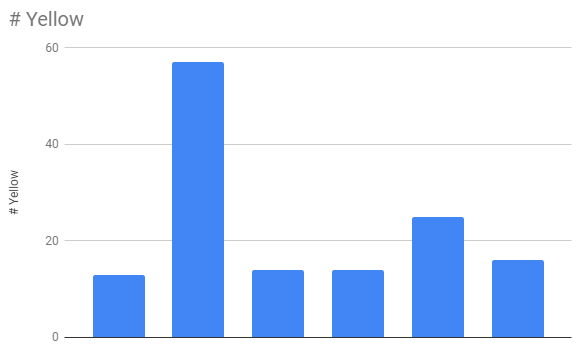
In a bar graph, the length of the bar for each category is proportional to the number or percent of individuals in each category. Bars may be vertical or horizontal.
Three graphs that are used to display quantitative data are dot plots, histograms, and box plots.
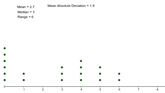
In a dot plot, individual dots are used to represent individual data values on a number line of values.
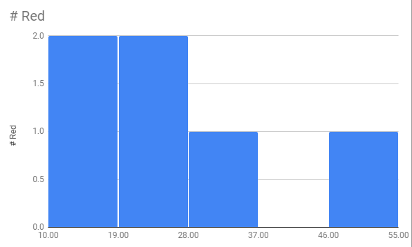
In a histogram, data is represented similarly to a bar graph in structure. However, there is usually no distance or space between the groups of data, called bins, which contain a range of data values instead of a single unique data value/description.
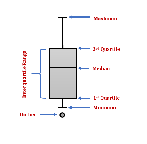
In a box plot (also called a box and whisker plot), a five-number summary is used to construct a visual display of the spread of the data. The five-number summary includes the minimum, the first quartile, the median, the third quartile, and the maximum.
It is a good idea to look at a variety of graphs to see which is the most helpful in displaying the data. We might make different choices of what we think is the “best” graph depending on the data and the context. Our choice also depends on what we are using the data for.
The Mean, Median, and Mode
The mean is often called the arithmetic average. It is computed by dividing the sum of the values by the number of values. Students want to know the mean of their test scores. Climatologists report that the mean temperature has, or has not, changed. City planners are interested in the mean household size.
The words “mean” and “average” are often used interchangeably. The substitution of one word for the other is common practice. The technical term is “arithmetic mean” and “average” is technically a center location. However, in practice among non-statisticians, “average” is commonly accepted for “arithmetic mean.”


Suppose Ethan’s first three test scores were 85, 88 and 94. To find the mean score, he would add them and divide them by 3.

His mean test score is 89 points.
The mean of a set of n numbers is the arithmetic average of the numbers.
- Write the formula for the mean

- Find the sum of all the values in the set. Write the sum in the numerator.
- Count the number, n, of values in the set. Write this number in the denominator.
- Simplify the fraction.
- Check to see that the mean is reasonable. It should be greater than the least number and less than the greatest number in the set.
Try it! – Finding the Mean
Find the mean of the numbers 8, 12, 15, 9, and 6.
Solution (click to reveal)
| Steps | Arithmetic |
|---|---|
| Write the formula for the mean: |  |
| Write the sum of the numbers in the numerator. |  |
| Count how many numbers are in the set. There are 5 numbers in the set, so n = 5. |  |
| Add the numbers in the numerator. |  |
| Then divide. |  |
| Check to see that the mean is ‘typical’: 10 is neither less than 6 nor greater than 15. |  |
It is customary to report the mean to one more decimal place than the original numbers. For example, if the numbers represent money, then it will make sense to report the mean in dollars and cents.
The “center” of a data set is also a way of describing location. The two most widely used measures of the “center” of the data are the mean (average) and the median. To calculate the mean weight of 50 people, add the 50 weights together and divide by 50. To find the median weight of the 50 people, order the data and find the number that splits the data into two equal parts. The median is generally a better measure of the center when there are extreme values or outliers because it is not affected by the precise numerical values of the outliers. The mean is the most common measure of the center.
The median of a set of data values is the middle value.
- Half the data values are less than or equal to the median.
- Half the data values are greater than or equal to the median.
How to: Find the Median
- List the numbers from smallest to largest.
- Count how many numbers are in the set. Call this n.
- Is n odd or even?
- If n is an odd number, the median is the middle value.
- If n is an even number, the median is the mean of the two middle values.
Try it! – Finding the Median
Find the median of 12, 13, 19, 9, 11, 15, and 18.
Solution (click to reveal)
| Steps | Arithmetic |
|---|---|
| List the numbers in order from smallest to largest. | 9, 11, 12, 13, 15, 18, 19 |
| Count how many numbers are in the set. Call this n. | n = 7 |
| Is n odd or even? | odd |
| The median is the middle value. | ![\[ \begin{array}{ccccccc} & & & \text{median} & & & \\ & & & \color{myblue1}\downarrow & & & \\ 9, & 11, & 12, & \textbf{13,} & 15, & 18, & 19 \\ \multicolumn{3}{c}{\color{myblue1}\underbrace{\phantom{0000000000}}} & & \multicolumn{3}{c}{\color{myblue1}\underbrace{\phantom{0000000000}}} \\ \multicolumn{3}{c}{\text{3 below}} & & \multicolumn{3}{c}{\text{3 above}} \end{array} \]](https://utsa.pressbooks.pub/app/uploads/quicklatex/quicklatex.com-1d663f4bad8314d80c4f9918dc022f01_l3.png "Rendered by QuickLaTeX.com") |
| The middle is the number in the 4th position. | So the median of the data is 13 |
Kristen received the following scores on her weekly math quizzes: 83, 79, 85, 86, 92, 100, 76, 90, 88, and 64. Find her median score.
Solution (click to reveal)
| Steps | Arithmetic |
|---|---|
| List the numbers in order from smallest to largest. | 64, 76, 79, 83, 85, 86, 88, 90, 92, 100 |
| Count the number of data values in the set. Call this n. | n = 10 |
| Is n odd or even? | even |
| The median is the mean of the two middle values, the 5th and 6th numbers. | ![\[ \begin{array}{cc} 64, 76, 79, 83, \mathbf{85}, & \mathbf{86}, 88, 90, 92, 100 \\ \color{myblue1}\underbrace{\phantom{000000000000000}} & \color{myblue1}\underbrace{\phantom{000000000000000}} \\ \text{5 numbers} & \text{5 numbers} \end{array} \]](https://utsa.pressbooks.pub/app/uploads/quicklatex/quicklatex.com-18d4c328f83082d258d310e45780b474_l3.png "Rendered by QuickLaTeX.com") |
| Find the mean of 85 and 86. | mean =  |
| Solution | mean = 85.5
Kristen’s median score is 85.5. |
Another measure of the center is the mode. The mode is the most frequent value. The frequency is the number of times a number occurs. So the mode of a set of numbers is the number with the highest frequency. There can be more than one mode in a data set as long as those values have the same frequency and that frequency is the highest. A data set with two modes is called bimodal.
The mode of a set of numbers is the number with the highest frequency.
How to: Find the Mode
- List the data values in numerical order.
- Count the number of times each value appears.
- The mode is the value with the highest frequency.
Try it! – Finding the Mode
Statistics exam scores for 20 students are as follows: 50, 53, 59, 59, 63, 63, 72, 72, 72, 72, 72, 76, 78, 81, 83, 84, 84, 84, 90, 93
Find the mode.
Solution (click to reveal)
The most frequent score is 72, which occurs five times.
Mode = 72.
The Five-Number Summary, Quartiles & Box Plots
The five-number summary is a set of measurements about the central tendencies of a set of data. These summaries are used to create boxplots that allow a good analysis of the spread of the data.
A description of the spread of a data set consists of the following aspects:
- Minimum Value
- First Quartile
- Median
- Third Quartile
- Maximum Value
The common measures of location are quartiles and percentiles.
Quartiles divide an ordered data set into four equal parts. The three quartiles of a data set are labeled as Q1, Q2, and Q3.
- About one-fourth of the data falls on or below the first quartile Q1.
- About one-half of the data falls on or below the second quartile Q2.
- About three-fourths of the data falls on or below the first quartile Q3.
As described above, the median is a number that measures the “center” of the data. You can think of the median as the “middle value,” but it does not actually have to be one of the observed values. It is a number that separates ordered data into halves. Half the values are the same number or smaller than the median, and half the values are the same number or larger.
Quartiles are numbers that separate the data into quarters. Quartiles may or may not be part of the data. To find the quartiles, first find the median or second quartile. The first quartile, Q1, is the middle value of the lower half of the data, and the third quartile, Q3, is the middle value, or median, of the upper half of the data. To get the idea, consider the data set:
1; 1; 2; 2; 4; 6; 6.8; 7.2; 8; 8.3; 9; 10; 10; 11.5
The median or second quartile is seven. The lower half of the data are 1, 1, 2, 2, 4, 6, 6.8. The middle value of the lower half is two.
The number two, which is part of the data, is the first quartile. One-fourth of the entire sets of values are the same as or less than two and three-fourths of the values are more than two.
The upper half of the data is 7.2, 8, 8.3, 9, 10, 10, 11.5. The middle value of the upper half is nine.
The third quartile, Q3, is nine. Three-fourths (75%) of the ordered data set are less than nine. One-fourth (25%) of the ordered data set are greater than nine. The third quartile is part of the data set in this example.
Try it! – Quartiles
Sharpe Middle School is applying for a grant that will be used to add fitness equipment to the gym. The principal surveyed 15 anonymous students to determine how many minutes a day the students spend exercising. The results from the 15 anonymous students are shown.
0 minutes; 40 minutes; 60 minutes; 30 minutes; 60 minutes; 10 minutes; 45 minutes; 30 minutes; 300 minutes; 90 minutes; 30 minutes; 120 minutes; 60 minutes; 0 minutes; 20 minutes
Determine the following five number values (the Min, max, Q1, Q2, and Q3 values).
Solution (click to reveal)
- Min = 0
- Q1 = 20
- Med = 40
- Q3 = 60
- Max = 300
A potential outlier is a data point that is significantly different from the other data points. These special data points may be errors or some kind of abnormality or they may be a key to understanding the data.
We will be using these elements of the 5-number summary to create Box plots.
Box plots
Box plots (also called box-and-whisker plots or box-whisker plots) give a good graphical image of the concentration of the data. They also show how far the extreme values are from most of the data. A box plot is constructed from five values: the minimum value, the first quartile, the median, the third quartile, and the maximum value. We use these values to compare how close other data values are to them.
To construct a box plot, use a horizontal or vertical number line and a rectangular box. The smallest and largest data values label the endpoints of the axis. The first quartile marks one end of the box and the third quartile marks the other end of the box. Quartiles are determined by splitting the data in half around its median value. The median of the “lower half” of the data will give you your first quartile. The median of the “upper half” of the split data will give you your third quartile. Approximately the middle 50 percent of the data falls inside the box. The “whiskers” extend from the ends of the box to the smallest and largest data values. The median or second quartile can be between the first and third quartiles, or it can be one, or the other, or both. The box plot gives a good, quick picture of the data.
You may encounter box-and-whisker plots that have dots marking outlier values. In those cases, the whiskers are not extended to the minimum and maximum values.
Consider, again, this dataset : 1, 1, 2, 2, 4, 6, 6.8, 7.2, 8, 8.3, 9, 10, 10, 11.5
The first quartile is two, the median is seven, and the third quartile is nine. The smallest value is one, and the largest value is 11.5. The following image shows the constructed box plot.
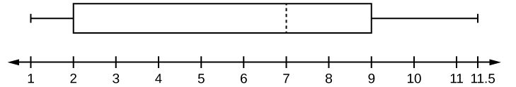
The two whiskers extend from the first quartile to the smallest value and from the third quartile to the largest value. The median is shown with a dashed line.
It is important to start a box plot with a scaled number line. Otherwise, the box plot may not be useful.
Try it! – Creating a Boxplot
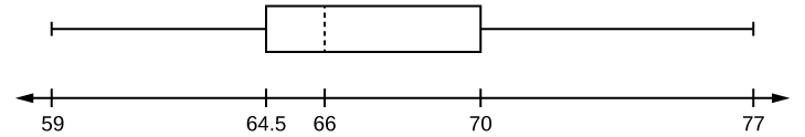
The following data are the heights of 40 students in a statistics class.
59; 60; 61; 62; 62; 63; 63; 64; 64; 64; 65; 65; 65; 65; 65; 65; 65; 65; 65; 66; 66; 67; 67; 68; 68; 69; 70; 70; 70; 70; 70; 71; 71; 72; 72; 73; 74; 74; 75; 77
First, calculate the Min, max, Q1, Q2, and Q3 values. Then construct a box plot .
Solution (click to reveal)
- Minimum value = 59
- Maximum value = 77
- Q1: First quartile = 64.5
- Q2: Second quartile or median= 66
- Q3: Third quartile = 70
- Each quarter has approximately 25% of the data.
- The spreads of the four quarters are 64.5 – 59 = 5.5 (first quarter), 66 – 64.5 = 1.5 (second quarter), 70 – 66 = 4 (third quarter), and 77 – 70 = 7 (fourth quarter). So, the second quarter has the smallest spread and the fourth quarter has the largest spread.
- Range = maximum value – the minimum value = 77 – 59 = 18
- Interquartile Range: IQR = Q3 – Q1 = 70 – 64.5 = 5.5.
- The interval 59 – 65 has more than 25% of the data so it has more data in it than the interval 66 through 70 which has 25% of the data.
- The middle 50% (middle half) of the data has a range of 5.5 inches.
Key Concepts
- Calculate the mean of a set of numbers.
- Write the formula for the

- Find the sum of all the values in the set. Write the sum in the numerator.
- Count the number, n, of values in the set. Write this number in the denominator.
- Simplify the fraction.
- Check to see that the mean is reasonable. It should be greater than the least number and less than the greatest number in the set.
- Write the formula for the
- Find the median of a set of numbers.
- List the numbers from least to greatest.
- Count how many numbers are in the set. Call this n.
- Is n odd or even?
If n is an odd number, the median is the middle value.
If n is an even number, the median is the mean of the two middle values
- Identify the mode of a set of numbers.
- List the data values in numerical order.
- Count the number of times each value appears.
- The mode is the value with the highest frequency.
- Derived from Openstax Introductory Statistics, Access for free at https://openstax.org/books/introductory-statistics-2e/pages/1-introduction. Pre-Algebra, Access for free at https://openstax.org/books/prealgebra-2e/pages/1-introduction ↵
a set of observations, or possible outcomes, whose value is indicated by a label
a set of observations, or possible outcomes, whose value is indicated by a number.
a variable whose outcomes are counted
a variable whose outcomes are measured
a ratio whose denominator is 100
the value that is the median of the lower half of the ordered data set.
The median of a set of data values is the middle value.
Half the data values are less than or equal to the median.
Half the data values are greater than or equal to the median.
the value that is the median of the upper half of the ordered data set
is the arithmetic average of the numbers. The formula is
mean = (sum of values in data set) / n
the number with the highest frequency
a graph that gives a quick picture of the middle 50% of the data
