13 Weighted Averages:
Topics Covered[1]
In case you missed something in class, or just want to review a specific topic covered in this Module, here is a list of topics covered:
Weighted Averages[2]
A weighted average is an average that has weights attached to the data values based on how important or relevant they are before taking the average. Not all data should be equally weighted when calculating the average. For example, when looking at poll numbers for politicians over various companies, a weighted average may be taken because sample size and date they were administered must be taken into account. A poll conducted two years ago is nowhere near as valid as one conducted last week, and a sample size of 100 is much less reliable than a size of 10,000. Your grade in your classes is a weighted average.
In a weighted average, some values contribute to the average more than others. This is often determined by how recent or significant the data value is. Any data value given a larger weight will affect the mean more intensely. Thus, when certain values are more weighted than others, the mean of the data can change.
The weights to use are usually provided to you, but in this class, if you are not given the weights to use, you can use the traditional numbering of 1 through the maximum number included in a group of data values.
It is important to remember that if decimal weights are being used, they must all add up to one in total. For example, three data values may be given the weights of 0.25, 0.40, and 0.35, because they all add up to 1.0.
Weighted moving averages often use the weighted averages formula, where you take the sum of the data values multiplied by their weights, and divided by the sum of the weights.

Where x = each data value, w = each weight value, and i is representing each instance in the data sequence, starting at 1. Σ represents the sum; meaning you add up all of the products of weights and data values.
Try it! – Weighted Average
Calculate the weighted mean of the grade a student would receive in their Mathematics course based on the following weights and item grades.
Solution
| Category | Weight | Score |
| Preview/Practice assignments average | 20% | 92 |
| Student Portfolio | 30% | 85 |
| Mini-Project average (Canvas) | 20% | 89 |
| Exams | 30% | 78 |
| Average: | ??? | ??? |
Each score should be multiplied by the weight associated with that category. First, each percent should be converted to decimal form.
| Category | Weight | Score |
| Preview/Practice assignments average | 0.20 | 92 |
| Student Portfolio | 0.30 | 85 |
| Mini-Project average (Canvas) | 0.20 | 89 |
| Exams | 0.30 | 78 |
| Average: | ??? | ??? |
Notice that all of the category weights add up to 100%, or 1.0. The category weight must be multiplied by the category score to get the weighted score.
| Category | Weighted Score |
|---|---|
| Preview/Practice assignments average | 0.20 * 92 |
| Student Portfolio | 0.30 * 85 |
| Mini-Project average (Canvas) | 0.20 * 89 |
| Exams | 0.30 * 78 |
| Average: | ??? |
| Category | Weighted Score |
|---|---|
| Preview/Practice assignments average | 18.4 |
| Student Portfolio | 25.5 |
| Mini-Project average (Canvas) | 17.8 |
| Exams | 23.4 |
| Average: | ??? |
To find the final midterm grade, you add together all the weights scores previously calculated and divide by the sum of the weights.
To find the sum of the weights to divide by, we would add all the weights together. As we discussed earlier, they all add up to 1.
 .
.
This means that whatever the sum of the weighted scores is, that is the final weighted average. This is because any number divided by 1 is itself.

| Category | Weighted Score |
|---|---|
| Preview/Practice assignments average | 18.4 |
| Student Portfolio | 25.5 |
| Mini-Project average (Canvas) | 17.8 |
| Exams | 23.4 |
| Average: | 85.1 |
When all of the weights scores are added together, you arrive at the overall weighted average. Each individual score is weighted differently based on the importance in the coursework.
Expected Value[3]
The expected value is often referred to as the “long-term” average or mean. This means that over the long term of doing an experiment over and over, you would expect this average.
You toss a coin and record the result. What is the probability that the result is heads? If you flip a coin two times, does probability tell you that these flips will result in one head and one tail? You might toss a fair coin ten times and record nine heads. As you learned, the probability does not describe the short-term results of an experiment. It gives information about what can be expected in the long term. To demonstrate this, Karl Pearson once tossed a fair coin 24,000 times! He recorded the results of each toss, obtaining heads 12,012 times. In his experiment, Pearson illustrated the Law of Large Numbers.
The Law of Large Numbers states that, as the number of trials in a probability experiment increases, the difference between the theoretical probability of an event and the relative frequency approaches zero (the theoretical probability and the relative frequency get closer and closer together). When evaluating the long-term results of statistical experiments, we often want to know the “average” outcome. This “long-term average” is known as the mean or expected value of the experiment and is denoted by the Greek letter μ. In other words, after conducting many trials of an experiment, you would expect this average value.
To find the expected value or long-term average, μ, multiply each value of the random variable by its probability and add the products.
Try it!
#1
A men’s soccer team plays soccer zero, one, or two days a week. The probability that they play zero days is 0.2, the probability that they play one day is 0.5, and the probability that they play two days is 0.3. Find the long-term average or expected value, μ, of the number of days per week the men’s soccer team plays soccer.
Solution
To do the problem, first, let the random variable X = the number of days the men’s soccer team plays soccer per week.  takes on the values 0, 1, 2. Construct a PDF table by adding a column
  . In this column, you will multiply each x value by its probability.
| x |  |
 |
|---|---|---|
| 0 | 0.2 | (0)(0.2) = 0 |
| 1 | 0.5 | (1)(0.5) = 0.5 |
| 2 | 0.3 | (2)(0.3) = 0.6 |
Add the last column to find the long-term average or expected value:

The expected value is 1.1. The men’s soccer team would, on average, expect to play soccer 1.1 days per week. The number 1.1 is the long-term average or expected value if the men’s soccer team plays soccer week after week after week. We say μ = 1.1.
#2
Suppose you play a game of chance in which five numbers are chosen from 0, 1, 2, 3, 4, 5, 6, 7, 8, 9. A computer randomly selects five numbers from zero to nine with replacement. You pay $2 to play and could profit $100,000 if you match all five numbers in order (you get your $2 back plus $100,000). Over the long term, what is your expected profit from playing the game?
Solution
To do this problem, set up an expected value table for the amount of money you can profit.
Let X = the amount of money you profit. The values of x are not 0, 1, 2, 3, 4, 5, 6, 7, 8, 9. Since you are interested in your profit (or loss), the values of x are 100,000 dollars and −2 dollars.
To win, you must get all five numbers correct, in order. The probability of choosing one correct number is  because there are ten numbers. You may choose a number more than once. The probability of choosing all five numbers correctly and in order is
 .
.
Therefore, the probability of winning is 0.00001, and the probability of losing is
 .
.
The expected value table is as follows:
| x | |
|
|
|---|---|---|---|
| Loss | –2 | 0.99999 | (–2)(0.99999) = – 1.99998 |
| Profit | 100,000 | 0.00001 | (100000)(0.00001) = 1 |

Since –0.99998 is about –1, you would, on average, expect to lose approximately $1 for each game you play. However, each time you play, you either lose $2 or profit $100,000. The $1 is the average or expected LOSS per game after playing this game over and over.
#3
Suppose you play a game with a biased coin. You play each game by tossing the coin once.  and
and  . If you toss a head, you pay $6. If you toss a tail, you win $10. If you play this game many times, will you come out ahead?
a. Define a random variable, X.
b. Complete the following expected value table.
| x | ____ | ____ | |
|---|---|---|---|
| WIN | 10 |  |
____ |
| LOSE | ____ | ____ |  |
c. What is the expected value, μ? Do you come out ahead?
Solution
a. X = amount of profit
b.
| x | |
|
|
|---|---|---|---|
| WIN | 10 | |
 |
| LOSE | –6 |  |
|
c. Add the last column of the table. The expected value  . You lose, on average, about 67 cents each time you play the game so you do not come out ahead.
#4
Find the expected value from the expected value table.
| x | |
|
|---|---|---|
| 2 | 0.1 | |
| 4 | 0.3 | |
| 6 | 0.4 | |
| 8 | 0.2 |
Solution
| x | |
|
|---|---|---|
| 2 | 0.1 | 2(0.1) = 0.2 |
| 4 | 0.3 | 4(0.3) = 1.2 |
| 6 | 0.4 | 6(0.4) = 2.4 |
| 8 | 0.2 | 8(0.2) = 1.6 |
The expected value is the sum of the products between the probability of an event and the event variable’s value:

Weighted Moving Averages[4]
When using a simple average, or the mean, of a data set, all data values are being given equal value. This makes sense when all of the individual data values are equally important, such as average temperature on a specific day or the average number of candies in bags produced in a day at a company production plant. However, there are certain situations where older data or data from smaller sample sizes would be considered less relevant. This is where the weighted average came in the previous module. Let’s suppose then that someone wanted to then look at the trends of change over extended periods of times of one of those instances requiring weighted averages. Maybe a student’s test scores over a semester? Do the sales change for a company over different financial quarters? How would that best be carried out? This is where the weighted moving average comes in handy. It allows for extended periods of data to be “smoothed” out so that overall trends and behavior can be determined and found within the instantaneous changes from data point to data point.
Weighted moving averages are weighted averages that “move” down sets of data. These moving averages allow for “jagged” data to be smoothed or straightened out so that it is easier to see overall trends of data over time.
A weighted moving average will take groups of values out of a data set, moving down the list of one data value at a time, and determine a weighted average for a group of values at each successive step through time. Just as in a normal weighted average, each value in the group is assigned a weighting based on the relevance or age of the data.
The number of data points to include in the groups is commonly three; but for this class, you will always be told how many data values to include in a group.
The weights to use are usually provided to you, but in this class, if you are not given the weights to use, you can use the traditional numbering of 1 through the maximum number included in a group of data values.
Weighted Moving Average Equation
Weighted moving averages still use the weighted averages formula, where you take the sum of the data values multiplied by their weights and divided by the sum of the weights.
Where x = each data value, w = each weight value, and i is representing each instance in the data sequence, starting at 1. Σ represents the sum; meaning you add up all of the products of weights and data values.
When filling in the weighted moving average values, you must be sure to start the data in the column number that matches the number of data values in the grouping. For example, if you are taking groups of four from your data set, the first moving average value will start in the weighted average column and in the fourth row. The following example illustrates this.
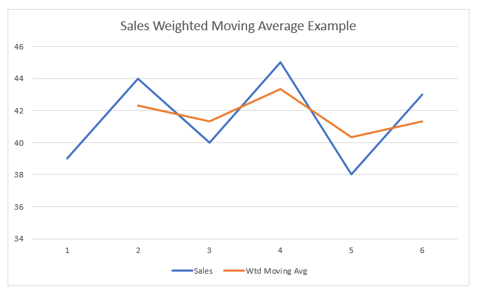
Try it! – Weighted Moving Average
For the following data, calculate the moving average for groups of two data points at a time. Use the traditional weights of 1 and 2 based on the most relevant data values.
| Week | Sales |
|---|---|
| 1 | 39 |
| 2 | 44 |
| 3 | 40 |
| 4 | 45 |
| 5 | 38 |
| 6 | 43 |
Solution
First, we must create a new column to fill in the moving averages.
| Week | Sales | Wtd Moving Average |
|---|---|---|
| 1 | 39 | |
| 2 | 44 | |
| 3 | 40 | |
| 4 | 45 | |
| 5 | 38 | |
| 6 | 43 |
Since we are taking groups of two, the first new data value will be a weighted average of week 1 and week 2 sales and will be placed in the second row of the last column. Because week 2 is more recent than week 1, week 2 gets the weighting of 2, and week 1 gets the weighting of 1.

Now, when we carry out the division, we must divide by the sum of the weights; which is  .
.

| Week | Sales | Wtd Moving Avg |
|---|---|---|
| 1 | 39 | |
| 2 | 44 | 42.33 |
| 3 | 40 | |
| 4 | 45 | |
| 5 | 38 | |
| 6 | 43 |


| Week | Sales | Wtd Moving Avg |
|---|---|---|
| 1 | 39 | |
| 2 | 44 | 42.33 |
| 3 | 40 | 41.33 |
| 4 | 45 | |
| 5 | 38 | |
| 6 | 43 |
| Week | Sales | Wtd Moving Avg |
|---|---|---|
| 1 | 39 | |
| 2 | 44 | 42.33 |
| 3 | 40 | 41.33 |
| 4 | 45 | 43.33 |
| 5 | 38 | 40.33 |
| 6 | 43 | 41.33 |
Using Spreadsheets for Calculating Statistics [5]
When working with data and statistics, there are often a lot of mathematical calculations that have to be carried out. Depending on how much data needs to be analyzed, it can become tenuous and time-consuming to compute needed statistics by hand. This is why most statistical analysis is done by the use of some kind of spreadsheet software.
In your course, you will be using Microsoft Excel a lot. Many of the calculations you will be expected to calculate can be easily entered into a cell and the program will do the math for you. The most important aspect of your skill, in this case, is knowing how to properly and efficient input data and utilizing the correct equations to complete your data analyses.
What follows are the many common equations and calculations you will be learning to do in the spreadsheet software you are using in this course.
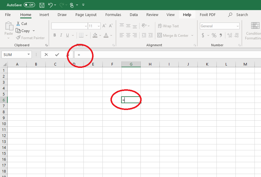
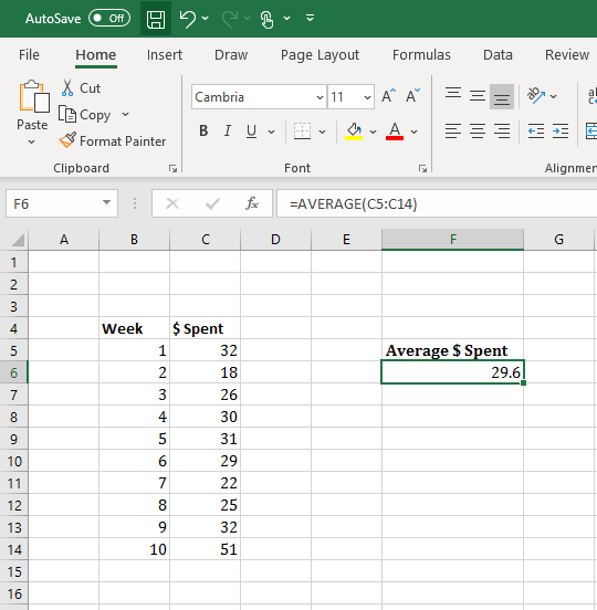
If you are having the spreadsheet calculate a statistic, it will not know to do so unless the first thing you enter is an equal sign. Anything else after the equal sign the spreadsheet will interpret as an equation or data to use in the equation you cite. When you finish the equation you want to type into the cell, you must hit the enter key for it to calculate the result.
Adding and Subtracting in Spreadsheet
When you need to add or subtract values, there are two options.
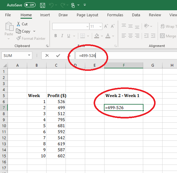
- Manually enter the numbers to be added with addition/subtraction signs included
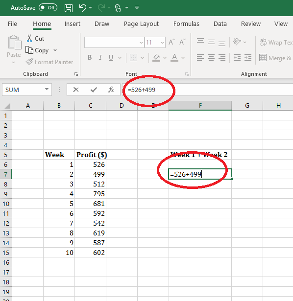
Adding by manually entering values.
- Clicking on cells that include the values that you want to add together with the addition/subtraction sign included
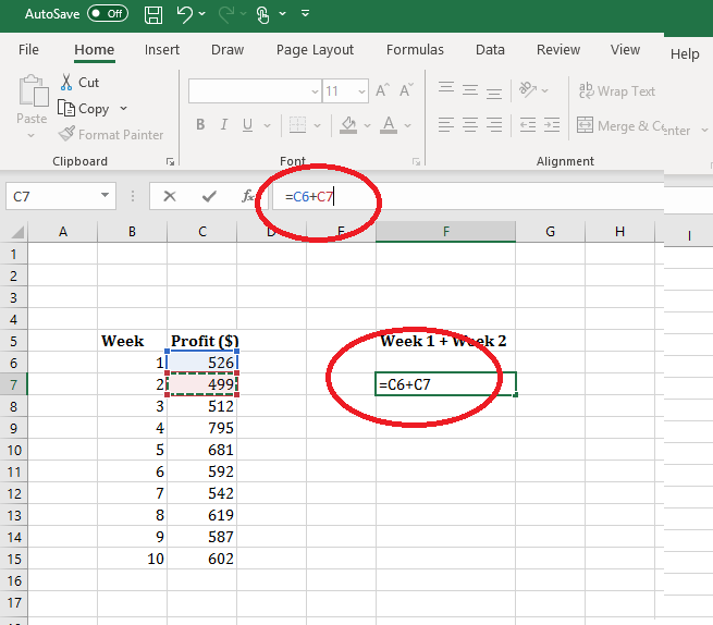
Adding by selecting cells with the values you want to add within them. Make sure to include the addition sign manually. 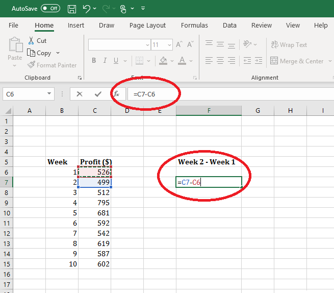
Subtracting by selecting cells with the values you want to subtract within them. Make sure to include the subtraction sign manually.
Multiplying and Dividing in Spreadsheet
In the spreadsheet programs you use, you may need to multiply or divide two numbers. Spreadsheets do not use regular multiplication or division symbols. Adding an x will not perform the multiplication function in spreadsheets.
For multiplication, you must use an asterisk * to complete multiplication between numbers. You can either:
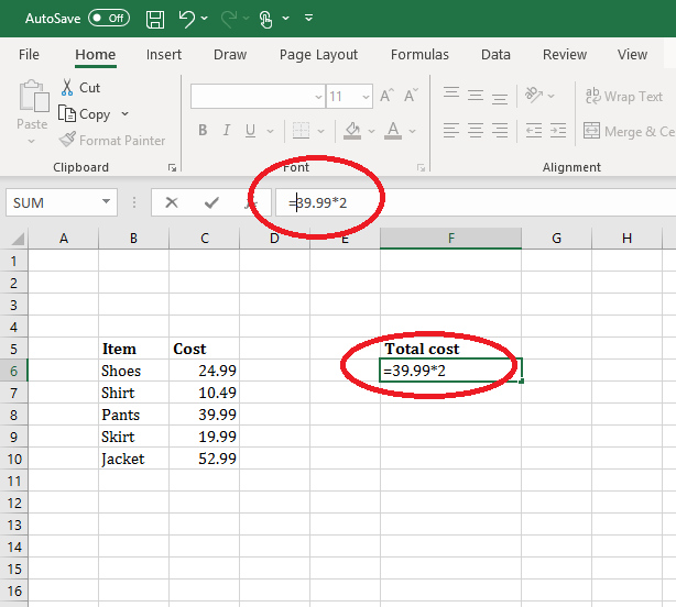
- Manually enter the values to be multiplied with an asterisk between them
- Click on the cells including the values you want to multiply together with an asterisk between them
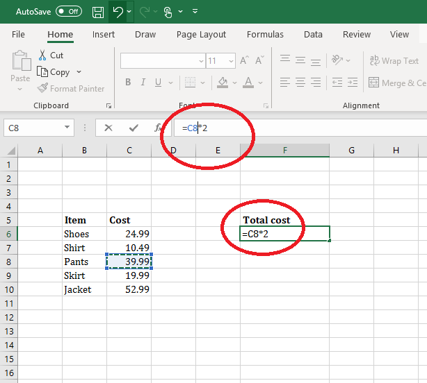
Multiplication by clicking on specific cell values with an asterisk for multiplication.
To complete division between two numbers. You can either:
- Manually enter the values to be divided with a backslash “/” between them
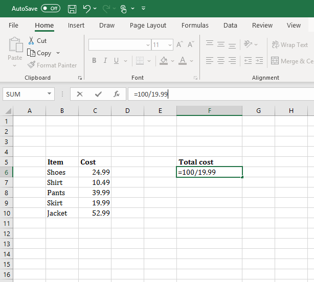
Division by manually entering values into a cell with a backslash for division. - Click on the cells including the values you want to divide together with a backslash between them
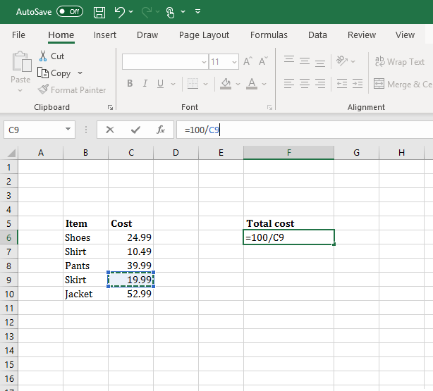
Division by clicking on specific cell values with a backslash for division.
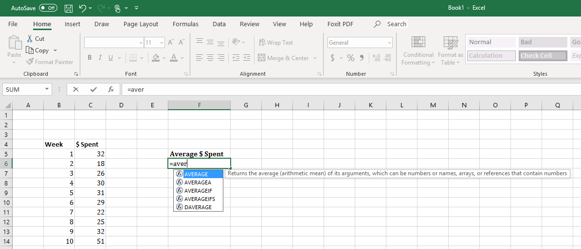
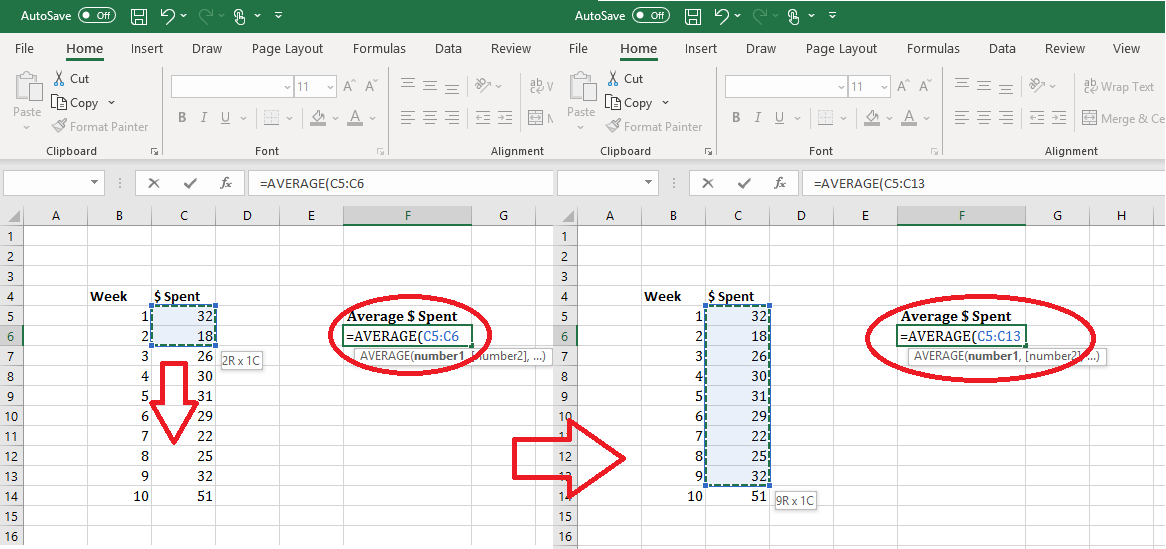
Utilizing Equations in Spreadsheets
Sometimes, you will need to use an equation in spreadsheets that aren’t simply adding/subtracting or multiplying/dividing. When needing to enter a specific equation, usually you can type the name of the equation into the cell after an equal sign “=” and a list will populate for you to choose from.
Key Concepts
- The weighted average is calculated as

- Mean or Expected Value:
![\displaystyle \mathbf{\[ \mu = \sum_{x \in X} x \cdot P(x)\]}](https://utsa.pressbooks.pub/app/uploads/quicklatex/quicklatex.com-afdad98852b3eec6b524bea2de13ec71_l3.png "Rendered by QuickLaTeX.com")
- The weighted moving average uses the weighted average equation and moves down a list of data one data value at a time.
- The weighted moving average can be used to “smooth out” data to visualize trends over time.
- Access for free at https://openstax.org/books/introductory-statistics-2e/pages/1-introduction ↵
- This material was created by Amanda Towry using the Microsoft Word processing program. ↵
- Section material derived from Openstax Introductory Statistics: Discrete Random Variables-Mean or Expected Value and Standard Deviation ↵
- This material was created by Amanda Towry using Microsoft Excel spreadsheet and Microsoft Word processing programs. ↵
- This material was created by Amanda Towry using the Microsoft Excel spreadsheets program. ↵
expected arithmetic average when an experiment is repeated many times; also called the mean. Notations: μ. For a discrete random variable (RV) with probability distribution function P(x),the definition can also be written in the form μ =∑xP(x).
As the number of trials in a probability experiment increases, the difference between the theoretical probability of an event and the relative frequency probability approaches zero.
A weighted average that moves through data one data value at a time to "smooth out" the data over time allowing for an easier identification of trends and habits of the data.
