18 Linear Relationships: Intro to Graphing
Topics Covered[1]
In case you missed something in class, or just want to review a specific topic covered in this Module, here is a list of topics covered:
Representations of Mathematical Data [2]
Often times when mathematical relationships or data need to be shared or presented, one of the most important decisions you will make will be on how you present your data. In mathematics, and in your Quantitative Reasoning course, there are four ways that data and information can and will be presented for interpretation.
Verbal Representation
A verbal representation is one where words are used to describe a mathematical problem, situation, or data set.
Mary has 5 red marbles, 3 blue marbles, and 7 green marbles. If Mary chooses two marble randomly from her collection out of a bag, what is the probability she will choose a red and a green one?
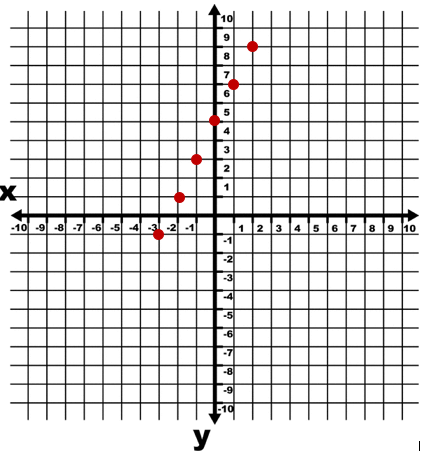
A numerical representation (sometimes called tabular) is one in which numbers describe or represent a mathematical problem, situation, or data set. It is most common to see a table for this type of representation.
| x | y |
| -3 | -1 |
| -2 | 1 |
| -1 | 3 |
| 0 | 5 |
| 1 | 7 |
| 2 | 9 |
| 3 | 11 |
A graphical representation is one in which mathematical information is plotted and generates a graph representing some relationship.
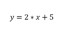
Symbolic/Algebraic Representation
A symbolic/algebraic representation is one in which mathematical information or relationships are presented using numbers and variables such as in an algebraic equation.
The next section will introduce how these are represented through Graphing and Linear equations.
The Rectangular Coordinate System[3]
The rectangular coordinate system is also called the x-y plane, the coordinate plane, or the Cartesian coordinate system (since it was developed by a mathematician named René Descartes.)
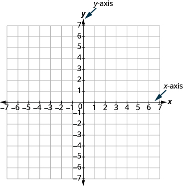
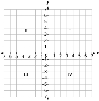
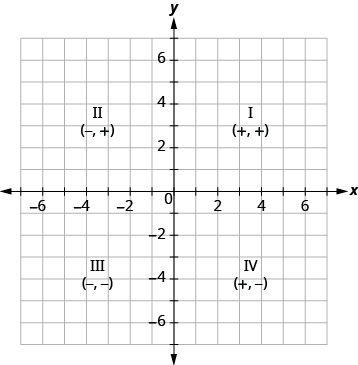
The x-axis and the y-axis form the rectangular coordinate system. These axes divide a plane into four areas, called quadrants. The quadrants are identified by Roman numerals, beginning on the upper right and proceeding counterclockwise. See the picture below.
<
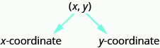
In the rectangular coordinate system, every point is represented by an ordered pair. The first number in the ordered pair is the x-coordinate of the point, and the second number is the y-coordinate of the point.
The point (0, 0) is called the origin. It is the point where the x-axis and y-axis intersect.
An ordered pair, (x, y) gives the coordinates of a point in a rectangular coordinate system.
We can summarize the sign patterns of the quadrants as follows.
| Quadrant I | Quadrant II | Quadrant III | Quadrant IV |
| (x, y) | (x, y) | (x, y) | (x, y) |
| (+, +) | (−, +) | (−, −) | (+, −) |
Try it! – Plotting Points in the Rectangular Coordinate System
Plot (1,3) and (3,1) in the same rectangular coordinate system.
Solution
| Steps | Graph |
| The coordinate values are the same for both points, but the x and y values are reversed. Let’s begin with point (1, 3). The x-coordinate is 1 so find 1 on the x-axis and sketch a vertical line through x = 1. The y-coordinate is 3 so we find 3 on the y-axis and sketch a horizontal line through y = 3. Where the two lines meet, we plot the point (1, 3). | 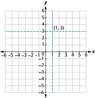 |
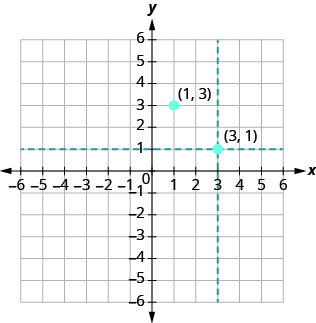
| To plot the point (3, 1), we start by locating 3 on the x-axis and sketch a vertical line through x = 3. Then we find 1 on the y-axis and sketch a horizontal line through y = 1. Where the two lines meet, we plot the point (3, 1).
Notice that the order of the coordinates does matter, so, (1, 3) is not the same point as (3, 1). |
 |
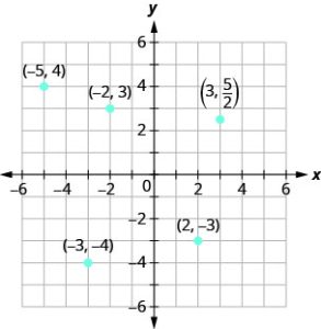
2.Plot each point in the rectangular coordinate system and identify the quadrant in which the point is located
a. (−5, 4) b.(−3, −4) c.(2, −3) d.(0,− 1) e.  .
.
Solution
The first number of the coordinate pair is the x-coordinate, and the second number is the y-coordinate. To plot each point, sketch a vertical line through the x-coordinate and a horizontal line through the y-coordinate. Their intersection is the point.
| Problem Number | Algebraic |
| a | Since x = −5, the point is to the left of the y-axis. Also, since y = 4, the point is above the x-axis. The point (−5, 4) is in Quadrant II. |
| b | Since x = −3, the point is to the left of the y-axis. Also, since y = −4, the point is below the x-axis. The point (−3, −4) is in Quadrant III. |
| c | Since x = 2, the point is to the right of the y-axis. Since y = −3, the point is below the x-axis. The point (2, −3) is in Quadrant IV. |
| d | Since x = 0, the point whose coordinates are (0, −1) is on the y-axis. |
| e | Since x = 3, the point is to the right of the y-axis. Since  , the point is above the x-axis. (It may be helpful to write , the point is above the x-axis. (It may be helpful to write  as a mixed number or decimal.) The point as a mixed number or decimal.) The point  )is in Quadrant I )is in Quadrant I |
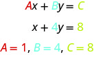
Equations with two variables may be of the form Ax + By = C. An equation of this form is called a linear equation in two variables.
Linear Equation
An equation of the form Ax + By = C, where A and B are not both zero, is called a linear equation in two variables.
Here is an example of a linear equation in two variables, x and y.
The equation y = −3x + 5 is also a linear equation. But it does not appear to be in the form Ax + By = C. We can use the Addition Property of Equality and rewrite it in Ax + By = C form.
|
Steps
|
Algebraic |
| y = −3x + 5 | |
| Add to both sides. | y + 3x = −3x + 5 + 3x |
| Simplify. | y + 3x = 5 |
| Use the Commutative Property to put it in Ax + By = C form. | 3x + y = 5 |
By rewriting y = −3x + 5 as 3x + y = 5, we can easily see that it is a linear equation in two variables because it is of the form Ax + By = C. When an equation is in the form Ax + By = C, we say it is in standard form of a linear equation.
Standard Form of Linear Equation
A linear equation is in standard form when it is written Ax + By = C.
Most people prefer to have A, B, and C be integers and A ≥ 0 when writing a linear equation in standard form, although it is not strictly necessary.
Linear equations have infinitely many solutions. For every number that is substituted for x there is a corresponding y value. This pair of values is a solution to the linear equation and is represented by the ordered pair (x, y). When we substitute these values of x and y into the equation, the result is a true statement, because the value on the left side is equal to the value on the right side.
An ordered pair (x, y) is a solution of the linear equation Ax + By = C, if the equation is a true statement when the x– and y-values of the ordered pair are substituted into the equation.
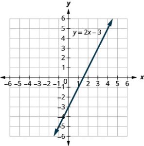
Linear equations have infinitely many solutions. We can plot these solutions in the rectangular coordinate system. The points will line up perfectly in a straight line. We connect the points with a straight line to get the graph of the equation. We put arrows on the ends of each side of the line to indicate that the line continues in both directions.
A graph is a visual representation of all the solutions of the equation. It is an example of the saying, “A picture is worth a thousand words.” The line shows you all the solutions to that equation. Every point on the line is a solution of the equation. And, every solution of this equation is on this line. This line is called the graph of the equation. Points not on the line are not solutions!
The graph of a linear equation Ax + By = C is a straight line.
- Every point on the line is a solution of the equation.
- Every solution of this equation is a point on this line.
Try it!
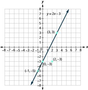
The graph of y = 2x − 3 is shown.
 For each ordered pair, decide:
a. Is the ordered pair a solution to the equation?
b. Are the following points on the line?
A: (0, −3) B: (3, 3) C: (2, −3) D: (−1, −5)
Solution
| Problem Number | Steps | Graph |
| a | Substitute the x– and y-values into the equation to check if the ordered pair is a solution to the equation. | 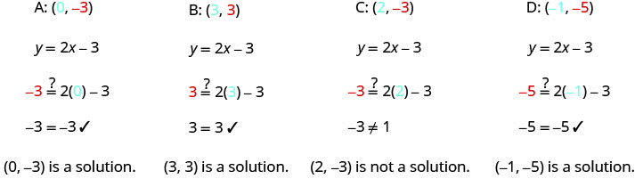 |
| b | Plot the points (0, −3), (3, 3), (2, −3), and (−1, −5).
The points (0, 3), (3, −3), and (−1, −5) are on the line y = 2x − 3, and the point (2, −3) is not on the line. |
 |
Graph a Linear Equation by Plotting Points[4]
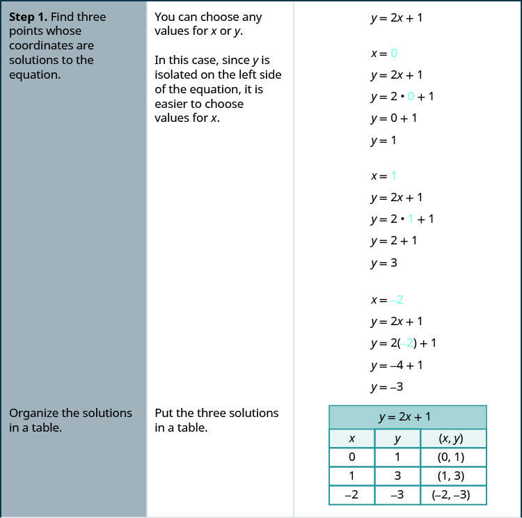
Let’s graph the equation y = 2x + 1 by plotting points.
We start by finding three points that are solutions to the equation. We can choose any value for x or y, and then solve for the other variable.
Since y is isolated on the left side of the equation, it is easier to choose values for x. We will use 0, 1, and -2 for x for this example. We substitute each value of x into the equation and solve for y.
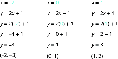
We can organize the solutions in a table.
| y = 2x + 1 | ||
|---|---|---|
| x | y | (x, y) |
| 0 | 1 | (0, 1) |
| 1 | 3 | (1, 3) |
| −2 | −3 | (−2, −3) |
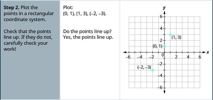
Now we plot the points on a rectangular coordinate system. Check that the points line up. If they did not line up, it would mean we made a mistake and should double-check all our work.
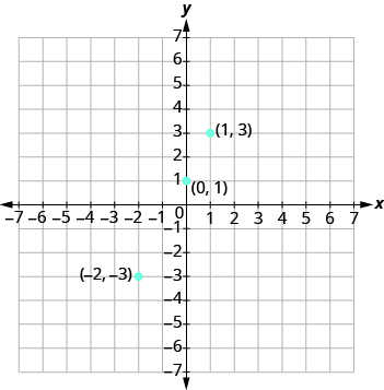
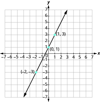
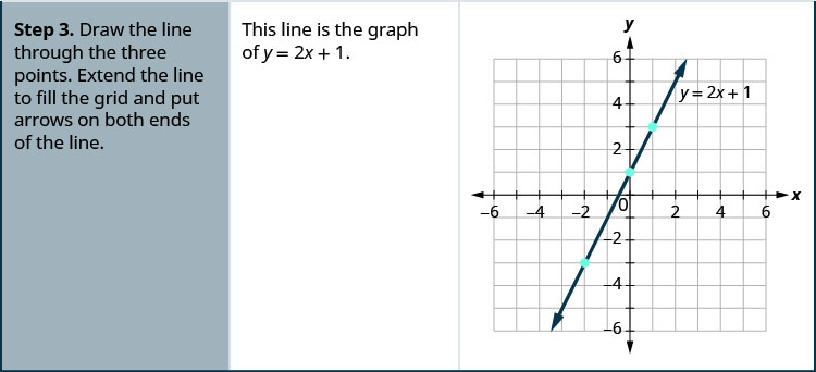
Draw the line through the three points. Extend the line to fill the grid and put arrows on both ends of the line. The line is the graph of y=2x+1.
How to graph a linear equation by plotting points:
- Find three points whose coordinates are solutions to the equation. Organize them in a table.
- Plot the points on a rectangular coordinate system. Check that the points line up. If they do not, carefully check your work.
- Draw the line through the points. Extend the line to fill the grid and put arrows on both ends of the line.
OR
How to graph by plotting points given an equation:
- Make a table with one column labeled x, a second column labeled with the equation, and a third column listing the resulting ordered pairs.
- Enter x-values down the first column using positive and negative values. Selecting the x-values in numerical order will make the graphing simpler.
- Select x-values that will yield y-values with little effort, preferably ones that can be calculated mentally.
- Plot the ordered pairs.
- Connect the points if they form a line.
Try it!
Graph the equation y = 2x + 1 by plotting points.
Try it! – Using Version 2 of the steps above
- Graph the equation y = −x + 2 by plotting points.
Solution
First, we construct a table. Then we choose x values and calculate y.
| x | y = −x + 2 | (x, y) |
|---|---|---|
| −5 | y = −(−5) + 2 = 7 | (−5, 7) |
| −3 | y = −(−3) + 2 = 5 | (−3, 5) |
| −1 | y = −(−1) + 2 = 3 | (−1, 3) |
| 0 | y = −(0) + 2 = 2 | (0, 2) |
| 1 | y = −(1) + 2 = 1 | (1, 1) |
| 3 | y = −(3) + 2 = −1 | (3, −1) |
| 5 | y = −(5) + 2 = −3 | (5, −3) |
Now, plot the points. Connect them if they form a line.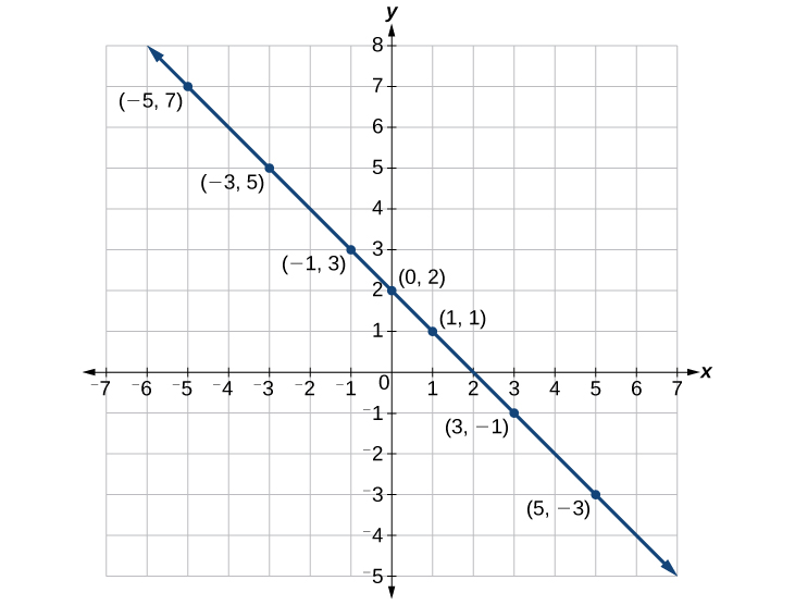
Graphing a Linear Equation with Intercepts[5]
Every linear equation has a unique line that represents all the solutions of the equation. When graphing a line by plotting points, each person who graphs the line can choose any three points, so two people graphing the line might use different sets of points.
At first glance, their two lines might appear different since they would have different points labeled. But if all the work was done correctly, the lines will be exactly the same line. One way to recognize that they are indeed the same line is to focus on where the line crosses the axes. Each of these points is called an intercept of the line.
Each of the points at which a line crosses the x-axis and the y-axis is called an intercept of the line.
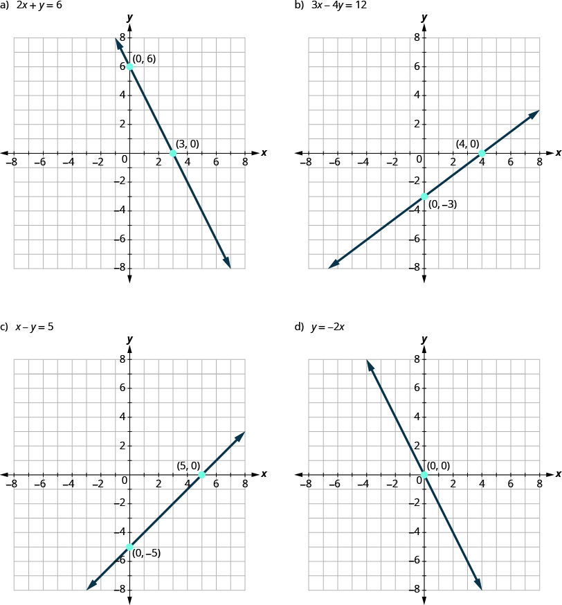
First, notice where each of these lines crosses the x-axis:
| Figure: | The line crosses the x-axis at: | Ordered pair of this point |
|---|---|---|
| Figure (a) | 3 | (3, 0) |
| Figure (b) | 4 | (4, 0) |
| Figure (c) | 5 | (5, 0) |
| Figure (d) | 0 | (0, 0) |
| General Figure | a | (a, 0) |
For each row, the y- coordinate of the point where the line crosses the x-axis is zero. The point where the line crosses the x-axis has the form (a,0); and is called the x-intercept of the line. The x-intercept occurs when y is zero.
Now, let’s look at the points where these lines cross the y-axis.
| Figure: | The line crosses the y-axis at: | Ordered pair for this point |
|---|---|---|
| Figure (a) | 6 | (0, 6) |
| Figure (b) | -3 | (0, -3) |
| Figure (c) | -5 | (0, -5) |
| Figure (d) | 0 | (0, 0) |
| General Figure | b | (0, b) |
For each row, the x- coordinate of the point where the line crosses the y-axis is zero. The point where the line crosses the y-axis has the form (0,b); and is called the y-intercept of the line. The y-intercept occurs when x is zero.
The x-intercept is the point, (a, 0), where the graph crosses the x-axis. The x-intercept occurs when y is zero.
The y-intercept is the point, (0, b), where the graph crosses the y-axis. The y-intercept occurs when x is zero.
To graph a linear equation by plotting points, you can use the intercepts as two of your three points. Find the two intercepts, and then a third point to ensure accuracy, and draw the line. This method is often the quickest way to graph a line.
How to Graph with Intercepts:
- Find the x- and y-intercepts of the line.
- Let y = 0 and solve for x
- Let x = 0 and solve for y.
- Find a third solution to the equation.
- Plot the three points and then check that they line up.
- Draw the line.
Try it! – Graphing with Intercepts
Graph −x + 2y = 6 using intercepts.
Solution
First, find the x-intercept. Let y = 0,

The x-intercept is (–6, 0).
Now find the y-intercept. Let x = 0.

The y-intercept is (0, 3).
Find a third point. We’ll use x = 2,

A third solution to the equation is (2, 4).
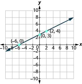
Summarize the three points in a table and then plot them on a graph.
| −x + 2y = 6 | ||
| x | y | (x, y) |
| −6 | 0 | (−6,0) |
| 0 | 3 | (0,3) |
| 2 | 4 | (2,4) |
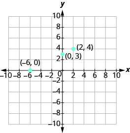
Do the points line up? Yes, so draw a line through the points.
Key Concepts
- Sign Patterns of the Quadrants
Quadrant I Quadrant II Quadrant III Quadrant IV (x, y) (x, y) (x, y) (x, y) (+, +) (−, +) (−, −) (+, −) - Coordinates of Zero
- Points with a y-coordinate equal to 0 are on the x-axis, and have coordinates (a, 0).
- Points with a x-coordinate equal to 0 are on the y-axis, and have coordinates (0, b).
- The point (0, 0) is called the origin. It is the point where the x-axis and y-axis intersect.
- Intercepts
- The x-intercept is the point, (a, 0), where the graph crosses the x-axis. The x-intercept occurs when y is zero.
- The y-intercept is the point, (0, b), where the graph crosses the y-axis. The y-intercept occurs when y is zero.
- The x-intercept occurs when y is zero.
- The y-intercept occurs when x is zero.
- Find the x and y intercepts from the equation of a line
- To find the x-intercept of the line, let y=0 and solve for x.
- To find the y-intercept of the line, let x=0 and solve for y.
x y 0 0
- Graph a line using the intercepts
- Find the x- and y- intercepts of the line.
- Let y = 0 and solve for x.
- Let x = 0 and solve for y.
- Find a third solution to the equation.
- Plot the three points and then check that they line up.
- Draw the line.
- Find the x- and y- intercepts of the line.
- Access for free at https://openstax.org/books/prealgebra-2e/pages/1-introduction ↵
- This material was created by Amanda Towry using the Microsoft Word processing program. ↵
- Section material derived from Openstax Prealgebra: The Properties of Real Numbers-Use the Rectangular Coordinate System ↵
- Section material derived from Openstax Prealgebra: Graphs-Understand Slope of a Line ↵
- Section material derived from Openstax Prealgebra: Graphs-Understand Slope of a Line ↵
A mathematical representation where words are used to describe the problem, situation, or data set.
A mathematical representation where the data or information is presented in numerical form such as in a data table.
A mathematical representation where the data or information is presented on a graph or coordinate place representing some relationship.
Each of the points at which a line crosses the x-axis and the y-axis is called an intercept of the line.
