Intro to Graphing

Elizabeth Pople

5 Intro to Graphing

Topics Covered

In case you missed something in class, or just want to review a specific topic covered in this Module, here is a list of topics covered:

Plot Points on a Rectangular Coordinate System

Just like maps use a grid system to identify locations, a grid system is used in algebra to show a relationship between two variables in a rectangular coordinate system. The rectangular coordinate system is also called the xy-plane or the “coordinate plane.”

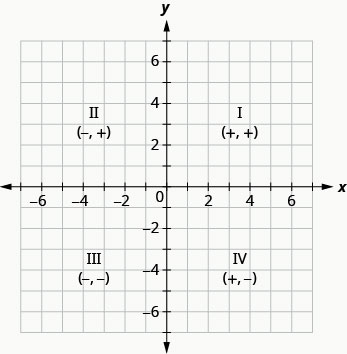
The rectangular coordinate system is formed by two intersecting number lines, one horizontal and one vertical. The horizontal number line is called the x-axis. The vertical number line is called the y-axis. These axes divide a plane into four regions, called quadrants. The quadrants are identified by Roman numerals, beginning on the upper right and proceeding counterclockwise. As shown in the figure below.

The signs of the x-coordinate and y-coordinate affect the location of the points. We can summarize the sign patterns of the quadrants in this way:

Quadrant I

Quadrant II

Quadrant III

Quadrant IV

(x ,y)

(x, y)

(x ,y)

(x, y)

(+, +)

(−, +)

(−, −)

(+, −)

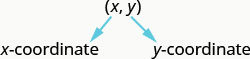
This figure shows the x y-coordinate plane with the four quadrants labeled. In the top right of the plane is quadrant I labeled (plus, plus). In the top left of the plane is quadrant II labeled (minus, plus). In the bottom left of the plane is quadrant III labeled (minus, minus). In the bottom right of the plane is quadrant IV labeled (plus, minus).

In the rectangular coordinate system, every point is represented by an ordered pair. The first number in the ordered pair is the x-coordinate of the point, and the second number is the y-coordinate of the point. The phrase “ordered pair” means that the order is important.

An ordered pair, (x , y) gives the coordinates of a point in a rectangular coordinate system. The first number is the x-coordinate. The second number is the y-coordinate.

This figure shows the expression (x, y). The variable x is labeled x-coordinate. The variable y is labeled y-coordinate.

What is the ordered pair of the point where the axes cross? At that point both coordinates are zero, so its ordered pair is (0, 0). The point (0, 0)has a special name. It is called the origin.

The point (0, 0) is called the origin. It is the point where the x-axis and y-axis intersect.

We use the coordinates to locate a point on the xy-plane. Let’s plot the point (1 , 3) as an example. First, locate 1 on the x-axis and lightly sketch a vertical line through x=1. Then, locate 3 on the y-axis and sketch a horizontal line through y=3. Now, find the point where these two lines meet—that is the point with coordinates (1,3).

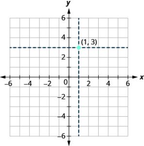This figure shows a point plotted on the x y-coordinate plane. The x and y axes run from negative 6 to 6. The point (1, 3) is labeled. A dashed vertical line goes through the point and intersects the x-axis at xplus1. A dashed horizontal line goes through the point and intersects the y-axis at yplus3. Notice that the vertical line through x = 1 and the horizontal line through y = 3 are not part of the graph. We just used them to help us locate the point (1, 3).

When one of the coordinates is zero, the point lies on one of the axes. As shown in the figure below, the point (0, 4) is on the y-axis and the point (−2, 0) is on the x-axis.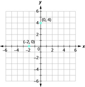 This figure shows points plotted on the x y-coordinate plane. The x and y axes run from negative 6 to 6. The point (negative 2, 0) is labeled and lies on the x-axis. The point (0, 4) is labeled and lies on the y-axis.

Points on the Axes

Points with a y-coordinate equal to 0 are on the x-axis, and have coordinates (a, 0).

Points with an x-coordinate equal to 0 are on the y-axis, and have coordinates (0, b).

Try it!

Plot each point in the rectangular coordinate system and identify the quadrant in which the point is located:

a. (−5, 4) b. (−3, −4) c. (2, −3) d. (0,− 1) e. $\displaystyle\left (3,\frac{5}{2}\right)$ .

Solution

The first number of the coordinate pair is the x-coordinate, and the second number is the y-coordinate. To plot each point, sketch a vertical line through the x-coordinate and a horizontal line through the y-coordinate. Their intersection is the point.

a. Since x = −5, the point is to the left of the y-axis. Also, since y = 4, the point is above the x-axis. The point (−5, 4) is in Quadrant II.

b. Since x = −3, the point is to the left of the y-axis. Also, since y = −4, the point is below the x-axis. The point (−3, −4) is in Quadrant III.

c. Since x = 2, the point is to the right of the y-axis. Since y = −3, the point is below the x-axis. The point (2, −3) is in Quadrant IV.

d. Since x = 0, the point whose coordinates are (0, −1) is on the y-axis.

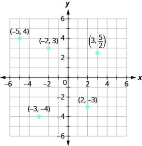
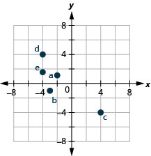
e. Since x = 3, the point is to the right of the y-axis. Since $\displaystyle y = \frac{5}{2}$ , the point is above the x-axis. (It may be helpful to write $\displaystyle\frac{5}{2}$ as a mixed number or decimal.) The point $\displaystyle\left (3, \frac{5}{2}\right)$ )is in Quadrant I This figure shows points plotted on the x y-coordinate plane. The x and y axes run from negative 6 to 6. The following points are labeled: (3, 5 divided by 2), (negative 2, 3), negative 5, 4), (negative 3, negative 4), and (2, negative 3).

Try it!

Plot each point in a rectangular coordinate system and identify the quadrant in which the point is located:

a. (−2, 1) b. (−3, −1) c. (4, −4) d. (−4, 4) e. (−4, 32)

Solution

This figure shows points plotted on the x y-coordinate plane. The x and y axes run from negative 6 to 6. The point labeled a is 2 units to the left of the origin and 1 unit above the origin and is located in quadrant II. The point labeled b is 3 units to the left of the origin and 1 unit below the origin and is located in quadrant III. The point labeled c is 4 units to the right of the origin and 4 units below the origin and is located in quadrant IV. The point labeled d is 4 units to the left of the origin and 4 units above the origin and is located in quadrant II. The point labeled e is 4 units to the left of the origin and 1 and a half units above the origin and is located in quadrant II.

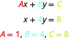
Up to now, all the equations you have solved were equations with just one variable. In almost every case, when you solved the equation you got exactly one solution. But equations can have more than one variable. Equations with two variables may be of the form Ax + By = C. An equation of this form is called a linear equation in two variables.

An equation of the form Ax + By = C, where A and B are not both zero, is called a linear equation in two variables.

Here is an example of a linear equation in two variables, x and y.

This figure shows the equation A x plus B y plus C. Below this is the equation x plus 4 y plus 8. Below this are the equations A plus 1, B plus 4, C plus 8. B and 4 are the same color in all the equations. C and 8 are the same color in all the equations.

The equation y = −3x + 5 is also a linear equation. But it does not appear to be in the form Ax + By = C. We can use the Addition Property of Equality and rewrite it in Ax + By = C form.

Steps

Algebraic

y = −3x + 5

Add to both sides.

y + 3x = −3x + 5 + 3x

Simplify.

y + 3x = 5

Use the Commutative Property to put it in Ax + By = C form.

3x + y = 5

By rewriting y = −3x + 5 as 3x + y = 5, we can easily see that it is a linear equation in two variables because it is of the form Ax + By = C. When an equation is in the form Ax + By = C, we say it is in standard form of a linear equation.

Standard Form of Linear Equation

A linear equation is in standard form when it is written Ax + By = C.

Most people prefer to have A, B, and C be integers and A ≥ 0 when writing a linear equation in standard form, although it is not strictly necessary.

Linear equations have infinitely many solutions. For every number that is substituted for x there is a corresponding y value. This pair of values is a solution to the linear equation and is represented by the ordered pair (x, y). When we substitute these values of x and y into the equation, the result is a true statement, because the value on the left side is equal to the value on the right side.

Solution of a Linear Equation in Two Variables

An ordered pair (x, y) is a solution of the linear equation Ax + By = C, if the equation is a true statement when the x– and y-values of the ordered pair are substituted into the equation.

Linear equations have infinitely many solutions. We can plot these solutions in the rectangular coordinate system. The points will line up perfectly in a straight line. We connect the points with a straight line to get the graph of the equation. We put arrows on the ends of each side of the line to indicate that the line continues in both directions.

A graph is a visual representation of all the solutions of the equation. It is an example of the saying, “A picture is worth a thousand words.” The line shows you all the solutions to that equation. Every point on the line is a solution of the equation. And, every solution of this equation is on this line. This line is called the graph of the equation. Points not on the line are not solutions!

The graph of a linear equation Ax + By = C is a straight line.

Every point on the line is a solution of the equation.
Every solution of this equation is a point on this line.

Try it!

The graph of y = 2x − 3 is shown.

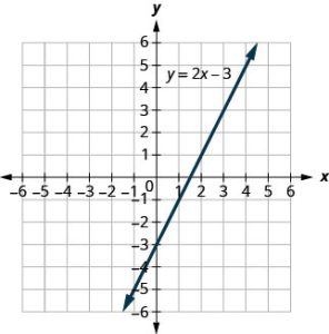This figure shows a straight line graphed on the x y-coordinate plane. The x and y-axes run from negative 10 to 10. The line has arrows on both ends and goes through the points (negative 3, negative 9), (negative 2, negative 7), (negative 1, negative 5), (0, negative 3), (1, negative 1), (2, 1), (3, 3), (4, 5), (5, 7), and (6, 9). The line is labeled y plus 2 x minus 3. For each ordered pair, decide:

a. Is the ordered pair a solution to the equation?

b. Are the following points on the line?

A: (0, −3) B: (3, 3) C: (2, −3) D: (−1, −5)

Solution

Substitute the x– and y-values into the equation to check if the ordered pair is a solution to the equation.

a.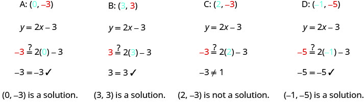b. Plot the points (0, −3), (3, 3), (2, −3), and (−1, −5). 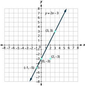This figure shows the graph of the linear equation y plus 2 x minus 3 and some points graphed on the x y-coordinate plane. The x and y-axes run from negative 10 to 10. The line has arrows on both ends and goes through the points (negative 1, negative 5), (0, negative 3), and (3, 3). The point (2, negative 3) is also plotted but not on the line. The points (0, 3), (3, −3), and (−1, −5) are on the line y = 2x − 3, and the point (2, −3) is not on the line.

The points that are solutions to y = 2x − 3 are on the line, but the point that is not a solution is not on the line.

Graph an Equation by Plotting Points

There are several methods that can be used to graph a linear equation. The first method we will use is called plotting points, or the Point-Plotting Method. We find three points whose coordinates are solutions to the equation and then plot them in a rectangular coordinate system. By connecting these points in a line, we have the graph of the linear equation.

Try it!

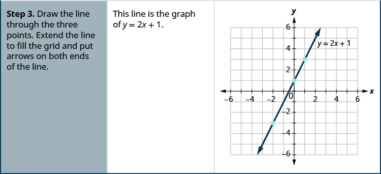
Graph the equation y = 2x + 1 by plotting points.

Solution:

Step 2 is to plot the points in a rectangular coordinate system. Plot: (0, 1), (1, 3), (negative 2, negative 3). The figure then shows a graph of some points plotted on the x y-coordinate plane. The x and y axes run from negative 6 to 6. The points (0, 1), (1, 3), and (negative 2, negative 3) are plotted. Check that the points line up. If they do not, carefully check your work! Do the point line up? Yes, the points in this example line up.

Step 3 is to draw the line through the three points. Extend the line to fill the grid and put arrows on both ends of the line. This line is the graph of y plus 2 x plus 1. The figure shows the graph of a straight line on the x y-coordinate plane. The x and y axes run from negative 6 to 6. The points (negative 2, negative 3), (0, 1), and (1, 3) are plotted. The straight line goes through the three points and has arrows on both ends.

How to graph a linear equation by plotting points.

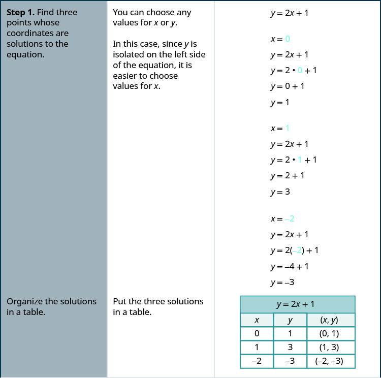
Find three points whose coordinates are solutions to the equation. Organize them in a table.
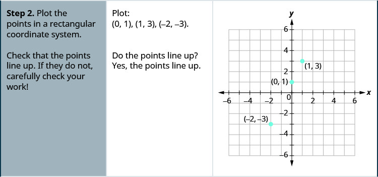
Plot the points in a rectangular coordinate system. Check that the points line up. If they do not, carefully check your work.
Draw the line through the three points. Extend the line to fill the grid and put arrows on both ends of the line.

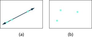
It is true that it only takes two points to determine a line, but it is a good habit to use three points. If you only plot two points and one of them is incorrect, you can still draw a line but it will not represent the solutions to the equation. It will be the wrong line.

If you use three points, and one is incorrect, the points will not line up. This tells you something is wrong and you need to check your work. Look at the difference between these illustrations.

The figure shows two images. In the first image there are three points with a straight line going through all three. In the second image there are three points that do not all lie on a straight line.

When an equation includes a fraction as the coefficient of x, we can still substitute any numbers for x. But the arithmetic is easier if we make “good” choices for the values of x. This way we will avoid fractional answers, which are hard to graph precisely.

Try it!

Graph the equation:

y = $\displaystyle\frac{1}{2}x+3$ .

Solution

Find three points that are solutions to the equation. Since this equation has the fraction $\displaystyle\frac{1}{2}$ as a coefficient of x, we will choose values of x carefully. We will use zero as one choice and multiples of 2 for the other choices. Why are multiples of two a good choice for values of x? By choosing multiples of 2 the multiplication by $\displaystyle\frac{1}{2}$ simplifies to a whole number.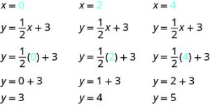The points are shown in the table below.

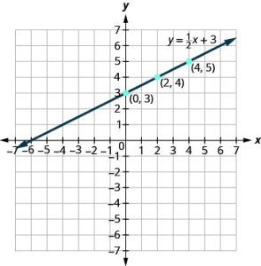
y = $\displaystyle\frac{1}{2}$ x + 3
x	y	(x, y)
0	3	(0, 3)
2	4	(2, 4)
4	5	(4, 5)

Plot the points, check that they line up, and draw the line.

The figure shows the graph of a straight line on the x y-coordinate plane. The x and y axes run from negative 7 to 7. The points (0, 3), (2, 4), and (4, 5) are plotted. The straight line goes through the three points and has arrows on both ends. The line is labeled y plus 1 divided by 2 times x plus 3.

What if the graph is NOT Linear?

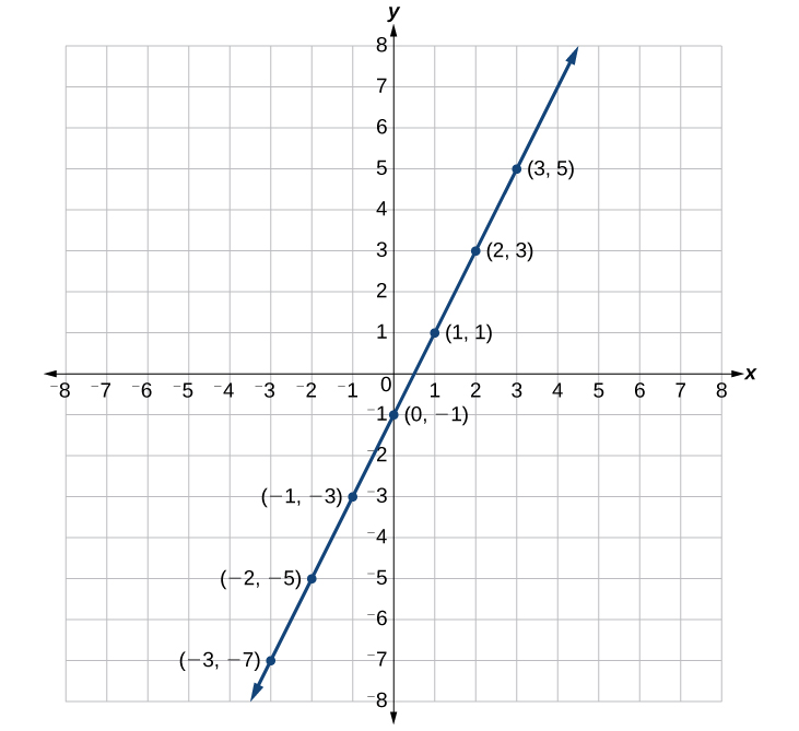
Suppose we want to graph the equation y = 2x − 1. We can begin by substituting a value for x into the equation and determining the resulting value of y. Each pair of x– and y-values is an ordered pair that can be plotted. The table lists values of x from –3 to 3 and the resulting values for y.

x

y = 2x − 1

(x, y)

−3

y = 2(−3) −1 = −7

(−3, −7)

−2

y = 2(−2) −1 = −5

(−2, −5)

−1

y = 2(−1) −1 = −3

(−1, −3)

0

y = 2(0) −1 = −1

(0, −1)

1

y = 2(1) − 1= 1

(1, 1)

2

y = 2(2) −1 = 3

(2, 3)

3

y = 2(3) −1 = 5

(3, 5)

We can plot the points in the table. The points for this particular equation form a line, so we can connect them. This is not true for all equations.

This is a graph of a line on an x, y coordinate plane. The x- and y-axis range from negative 8 to 8. A line passes through the points (-3, -7); (-2, -5); (-1, -3); (0, -1); (1, 1); (2, 3); and (3, 5).

Note that the x-values chosen are arbitrary, regardless of the type of equation we are graphing. Of course, some situations may require particular values of x to be plotted in order to see a particular result. Otherwise, it is logical to choose values that can be calculated easily, and it is always a good idea to choose values that are both negative and positive. There is no rule dictating how many points to plot, although we need at least two to graph a line. Keep in mind, however, that the more points we plot, the more accurately we can sketch the graph.

How to graph by plotting points given an equation.

Make a table with one column labeled x, a second column labeled with the equation, and a third column listing the resulting ordered pairs.
Enter x-values down the first column using positive and negative values. Selecting the x-values in numerical order will make the graphing simpler.
Select x-values that will yield y-values with little effort, preferably ones that can be calculated mentally.
Plot the ordered pairs.
Connect the points if they form a line.

Try it!

Graph the equation y = −x + 2 by plotting points.

Solution

First, we construct a table. Then we choose x values and calculate y.

x

y = −x + 2

(x, y)

−5

y = −(−5) + 2 = 7

(−5, 7)

−3

y = −(−3) + 2 = 5

(−3, 5)

−1

y = −(−1) + 2 = 3

(−1, 3)

0

y = −(0) + 2 = 2

(0, 2)

1

y = −(1) + 2 = 1

(1, 1)

3

y = −(3) + 2 = −1

(3, −1)

5

y = −(5) + 2 = −3

(5, −3)

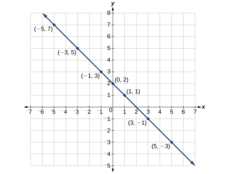
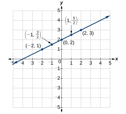
Now, plot the points. Connect them if they form a line. This image is a graph of a line on an x, y coordinate plane. The x-axis includes numbers that range from negative 7 to 7. The y-axis includes numbers that range from negative 5 to 8. A line passes through the points: (-5, 7); (-3, 5); (-1, 3); (0, 2); (1, 1); (3, -1); and (5, -3).

Try it!

Construct a table and graph the equation by plotting points: $\displaystyle y = \frac{1}{2}x + 2$ .

Solution

x

Algebraic

(x, y)

x

$\displaystyle y = \frac{1}{2}x + 2$

(x, y)

−2

$\displaystyle y = \frac{1}{2}(−2) + 2 = 1$

(−2, 1)

−1

$\displaystyle y = \frac{1}{2}$ (−1) + 2 = $\displaystyle\frac{3}{2}$

(−1, $\displaystyle\frac{3}{2}$ )

0

y = $\displaystyle\frac{1}{2}$ (0) + 2 = 2

(0, 2)

1

y = $\displaystyle\frac{1}{2}$ (1) + 2= $\displaystyle\frac{5}{2}$

(1, $\displaystyle\frac{5}{2}$ )

2

y = $\displaystyle\frac{1}{2}$ (2) + 2 = 3

(2, 3)

This is an image of a graph on an x, y coordinate plane. The x and y-axis range from negative 5 to 5. A line passes through the points (-2, 1); (-1, 3/2); (0, 2); (1, 5/2); and (2, 3).

Find x and y Intercepts

The intercepts of a graph are points at which the graph crosses the axes. The x-intercept is the point at which the graph crosses the x-axis. At this point, the y-coordinate is zero. The y-intercept is the point at which the graph crosses the y-axis. At this point, the x-coordinate is zero.

Let’s look at the graphs of the lines.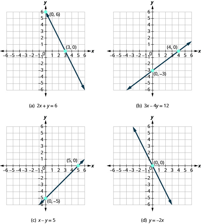First, notice where each of these lines crosses the x-axis. Now, let’s look at the points where these lines cross the y-axis.

Figure	The line crosses the x-axis at:	Ordered pair for this point	The line crosses the y-axis at:	Ordered pair for this point
Figure (a)	3	(3 ,0)	6	(0, 6)
Figure (b)	4	(4, 0)	−3	(0, −3)
Figure (c)	5	(5, 0)	−5	(0, 5)
Figure (d)	0	(0, 0)	0	(0, 0)
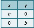
General Figure	a	(a, 0)	b	(0, b)

Do you see a pattern?

For each line, the y-coordinate of the point where the line crosses the x-axis is zero. The point where the line crosses the x-axis has the form (a, 0) and is called the x-intercept of the line. The x-intercept occurs when y is zero.

In each line, the x–coordinate of the point where the line crosses the y-axis is zero. The point where the line crosses the y-axis has the form (0, b) and is called the y-intercept of the line. The y-intercept occurs when x is zero.

x-intercept and y-intercept of a Line

The x-intercept is the point (a, 0) where the line crosses the x-axis. Occurs when y is zero.

The y-intercept is the point (0, b) where the line crosses the y-axis. Occurs when x is zero.

The table has 3 rows and 2 columns. The first row is a header row with the headers x and y. The second row contains a and 0. The third row contains 0 and b.

Try it!

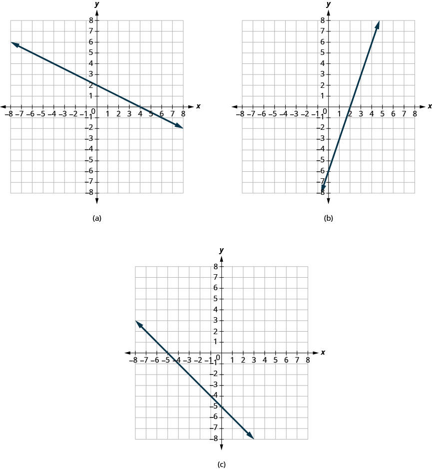
Find the x– and y-intercepts on each graph shown.

Solution

a. The graph crosses the x-axis at the point (4, 0). The x-intercept is (4, 0).
The graph crosses the y-axis at the point (0, 2). The y-intercept is (0, 2).

b. The graph crosses the x-axis at the point (2, 0). The x-intercept is (2, 0).
The graph crosses the y-axis at the point (0, −6). The y-intercept is (0, −6).

c. The graph crosses the x-axis at the point (−5, 0). The x-intercept is (−5, 0).
The graph crosses the y-axis at the point (0, −5). The y-intercept is (0, −5).

Key Concepts

Points on the Axes
- Points with a y-coordinate equal to 0 are on the x-axis, and have coordinates
  (a, 0).
- Points with an x-coordinate equal to
  0 are on the y-axis, and have coordinates(0, b).
Quadrant

Quadrant I

Quadrant II

Quadrant III

Quadrant IV

(x, y)

(+, +)

(−, +)

(−, −)

(+, −)

This figure shows the x y-coordinate plane with the four quadrants labeled. In the top right of the plane is quadrant I labeled (plus, plus). In the top left of the plane is quadrant II labeled (minus, plus). In the bottom left of the plane is quadrant III labeled (minus, minus). In the bottom right of the plane is quadrant IV labeled (plus, minus).

Graph of a Linear Equation: The graph of a linear equation Ax + By = C is a straight line.
Every point on the line is a solution of the equation.
Every solution of this equation is a point on this line.
How to graph a linear equation by plotting points.
1. Find three points whose coordinates are solutions to the equation. Organize them in a table.
2. Plot the points in a rectangular coordinate system. Check that the points line up. If they do not, carefully check your work.
3. Draw the line through the three points. Extend the line to fill the grid and put arrows on both ends of the line.
x-intercept and y-intercept of a Line
- The x-intercept is the point
  (a, 0) where the line crosses the x-axis.
- The y-intercept is the point
  (0, b) where the line crosses the y-axis.

License

Icon for the Creative Commons Attribution-NonCommercial-ShareAlike 4.0 International License

NCB 0502 - Support for Corequisite Algebra Copyright © by Elizabeth Pople is licensed under a Creative Commons Attribution-NonCommercial-ShareAlike 4.0 International License, except where otherwise noted.

Plot Points on a Rectangular Coordinate System

Graph an Equation by Plotting Points

Find x and y Intercepts

License

Share This Book