24 Polynomial Functions
Topics Covered
Recall earlier, we introduced Polynomials. Here is a brief review:
A polynomial is a sum of or difference of terms, each consisting of a variable raised to a nonnegative integer power. A number multiplied by a variable raised to an exponent, such as 384π, is known as a coefficient. Coefficients can be positive, negative, or zero and can be whole numbers, decimals, or fractions. Each product aixi, such as 384πw, is a term of a polynomial. If a term does not contain a variable, it is called a constant.
A polynomial containing only one term, such as 5x4, is called a monomial. A polynomial containing two terms, such as 2x – 9, is called a binomial. A polynomial containing three terms, such as -3x2 + 8x – 7, is called a trinomial.
Here are some examples of polynomials.
| Example | ||||
| Polynomial | y + 1 | 4a2 – 7ab + 2b2 | 4x4 + x3 + 8x2 – 9x + 1 | |
| Monomial | 14 | 8y2 | -9x3y5 | -13a3b2c |
| Binomial | a + 7b | 4x2 – y2 | y2 – 16 | 3p3q – 9p2q |
| Trinomial | x2 – 7x + 12 | 9m2 + 2mn – 8n2 | 6k4 – k3 + 8k | z4 + 3z2 – 1 |
Degree of a Polynomial
The degree of a term is the sum of the exponents of its variables.
The degree of a constant is 0.
The degree of a polynomial is the highest degree of all its terms.
Here are some additional examples.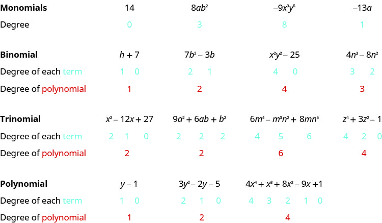 Working with polynomials is easier when you list the terms in descending order of degrees. When a polynomial is written this way, it is said to be in standard form of a polynomial. Get in the habit of writing the term with the highest degree first.
We can find the degree of a polynomial by identifying the highest power of the variable that occurs in the polynomial. The term with the highest degree is called the leading term because it is usually written first. The coefficient of the leading term is called the leading coefficient. When a polynomial is written so that the powers are descending, we say that it is in standard form.
 The same process can be applied to polynomial functions.
A polynomial function consists of either zero or the sum of a finite number of non-zero terms, each of which is a product of a number, called the coefficient of the term, and a variable raised to a non-negative integer power.
Polynomial Functions
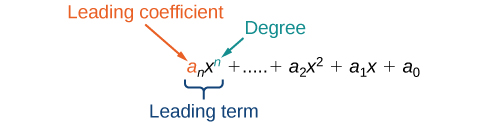
Let n be a non-negative integer. A polynomial function is a function that can be written in the form
f(x) = anxn + … + a2x2 + a1x + a0
This is called the general form of a polynomial function. Each ai is a coefficient and can be any real number, but a cannot = 0. Each expression aixi is a term of a polynomial function. The number a0 that is not multiplied by a variable is called a constant.
Try it! – Identifying Polynomial Functions
Which of the following are polynomial functions?

Solution:
The first two functions are examples of polynomial functions because they can be written in the form f(x) = anxn + … + a2x2 + a1x + a0, where the powers are non-negative integers and the coefficients are real numbers.
- f(x) can be written as f(x) = 6x4 + 4.
- g(x) can be written as g(x) = -x3 + 4x.
- h(x) cannot be written in this form and is therefore not a polynomial function.
Remember, like we discussed above, although the order of the terms in the polynomial function is not important for performing operations, we typically arrange the terms in descending order of power or in general form. The degree of the polynomial is the highest power of the variable that occurs in the polynomial; it is the power of the first variable if the function is in general form. The leading term is the term containing the highest power of the variable or the term with the highest degree. The leading coefficient is the coefficient of the leading term.
Terminology of Polynomial Functions
We often rearrange polynomials so that the powers are descending.
When a polynomial is written in this way, we say that it is in general form.
How to identify the degree and leading coefficient of a polynomial function.
- Find the highest power of x to determine the degree function.
- Identify the term containing the highest power of x to find the leading term.
- Identify the coefficient of the leading term.
Try it!
Identify the degree, leading term, and leading coefficient of the following polynomial functions.

Solution:
For the function f(x), the highest power of x is 3, so the degree is 3. The leading term is the term containing that degree, –4x3. The leading coefficient is the coefficient of that term, -4.
For the function g(t), the highest power of t is 5, so the degree is 5. The leading term is the term containing that degree, 5t5. The leading coefficient is the coefficient of that term, 5.
For the function h(p), the highest power of p is 3, so the degree is 3. The leading term is the term containing that degree, -p3. The leading coefficient is the coefficient of that term, -1.
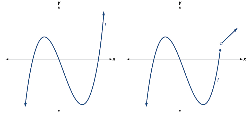
Polynomial functions of degree 2 or more have graphs that do not have sharp corners; these types of graphs are called smooth curves. Polynomial functions also display graphs that have no breaks. Curves with no breaks are called continuous. The figure below shows a graph of a polynomial function and a graph of a function that is not a polynomial.
Try it! – Recognizing Polynomial Functions
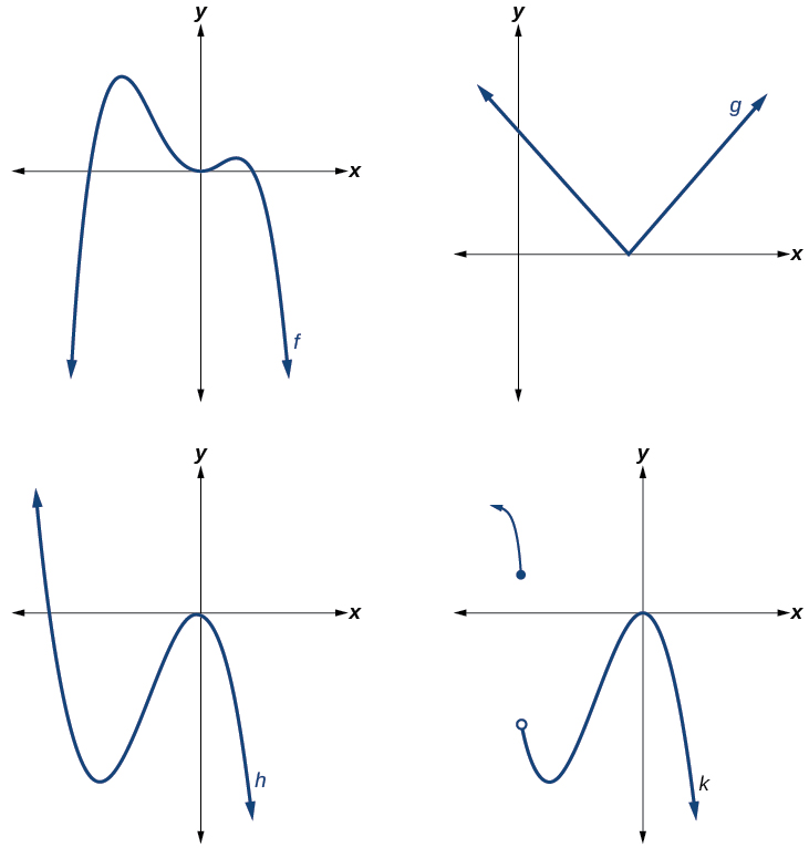
Which of the graphs below represents a polynomial function?
Solution:
The graphs of f and h are graphs of polynomial functions. They are smooth and continuous.
The graphs of g and k are graphs of functions that are not polynomials. The graph of function g has a sharp corner. The graph of function k is not continuous.
The behavior of the graph of a function as the input values get very small (x → -∞) and get very large (x → ∞) is referred to as the end behavior of the function. We can use words or symbols to describe end behavior. To describe the behavior as numbers become larger and larger, we use the idea of infinity. We use the symbol ∞ for positive infinity and -∞ for negative infinity. When we say that “x approaches infinity,” which can be symbolically written as x → ∞, we are describing a behavior; we are saying that x is increasing without bound.
Knowing the degree of a polynomial function is useful in helping us predict its end behavior. To determine its end behavior, look at the leading term of the polynomial function. Because the power of the leading term is the highest, that term will grow significantly faster than the other terms as x gets very large or very small, so its behavior will dominate the graph. For any polynomial, the end behavior of the polynomial will match the end behavior of the leading term.
| Polynomial Function | Leading Term | Graph of Polynomial Function |
|---|---|---|
| f(x) = 5x4 + 2x3 – x – 4 | 5x4 | 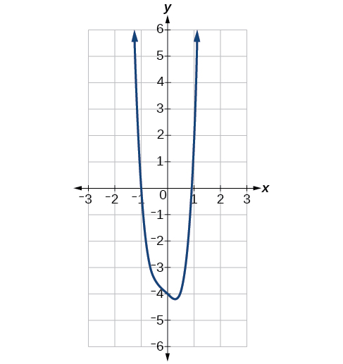 |
| f(x) = – 2x6 – x5 + 3x4 + x3 | -2x6 | 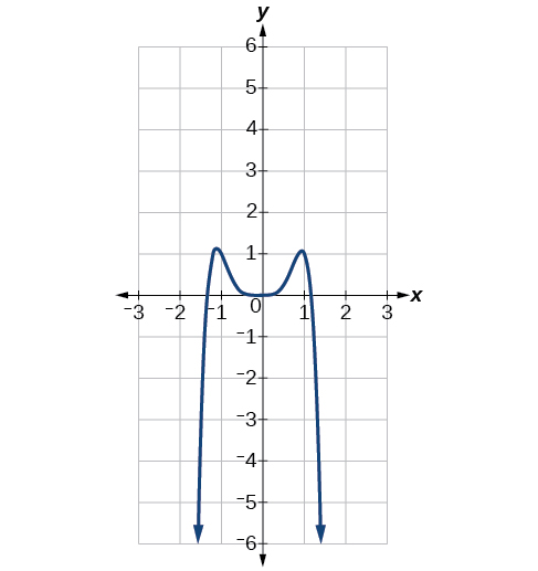 |
| f(x) = 3x5 – 4x4 +2x2 + 1 | 3x5 | 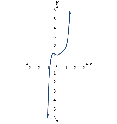 |
| f(x) = -6x3 + 7x2 + 3x + 1 | -6x3 | 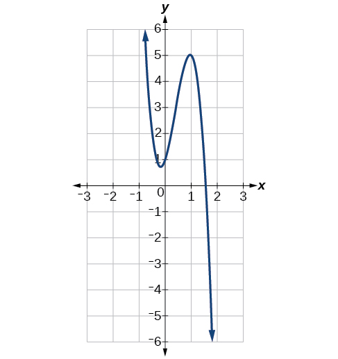 |
As we pointed out when discussing quadratic equations, when the leading term of a polynomial function, anxn, is an even power function, as x increases or decreases without bound, f(x) increases without bound. When the leading term is an odd power function, as x decreases without bound, f(x) also decreases without bound; as x increases without bound, f(x) also increases without bound. If the leading term is negative, it will change the direction of the end behavior. The table below summarizes all four cases.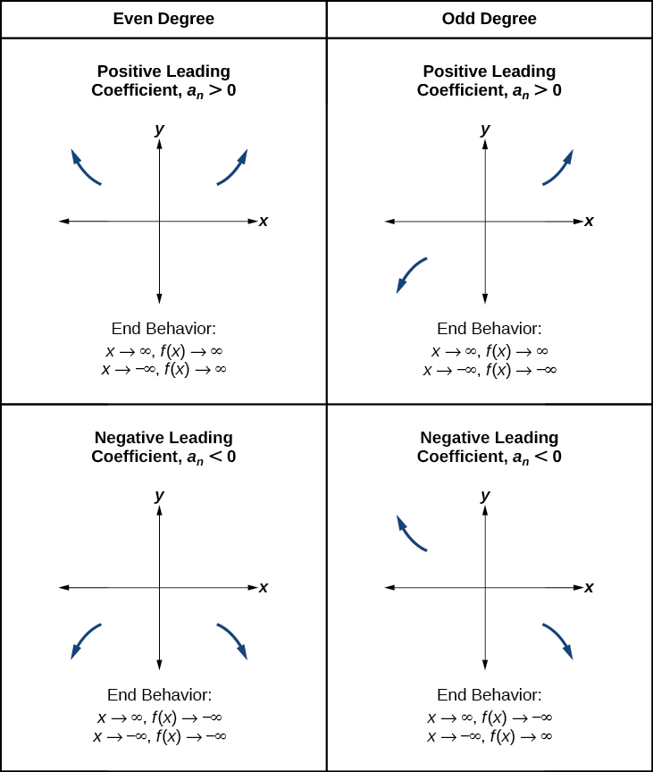
Try it! – Identifying End Behavior and Degree of a Polynomial Function
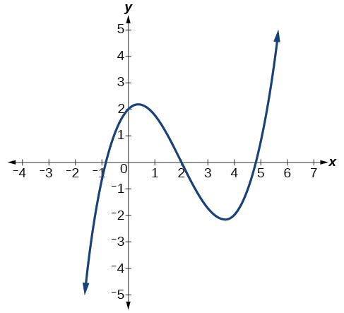
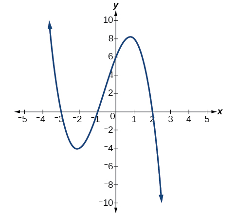
1. Describe the end behavior and determine a possible degree of the polynomial function represented by the graph below.
Solution:
As the input values x get very large, the output values f(x) increase without bound. As the input values x get very small, the output values f(x) decrease without bound. We can describe the end behavior symbolically by writing
as x → −∞, f(x) → −∞
as x → ∞, f(x) → ∞
In words, we could say that as x values approach infinity, the function values approach infinity, and as x values approach negative infinity, the function values approach negative infinity.
We can tell this graph has the shape of an odd degree power function that has not been reflected, so the degree of the polynomial creating this graph must be odd and the leading coefficient must be positive.
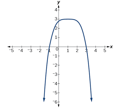
2. Describe the end behavior, and determine a possible degree of the polynomial function represented by the graph below.
Solution:
As x → ∞, f(x)→−∞; as x → −∞, f(x)→−∞.
It has the shape of an even degree power function with a negative coefficient.
3. Given the function f(x) = -3x2(x – 1)(x + 4), express the function as a polynomial in general form, and determine the leading term, degree, and end behavior of the function.
Solution:
Obtain the general form by expanding the given expression for f(x).

The general form is f(x) = -3x4 – 9x3 + 12x2. The leading term is -3x4; therefore, the degree of the polynomial is 4. The degree is even (4) and the leading coefficient is negative (–3), so the end behavior is
as x → -∞, f(x) → -∞
as x → ∞, f(x) → -∞
4. Given the function f(x) = 0.2(x – 2)(x + 1)(x – 5), express the function as a polynomial in general form and determine the leading term, degree, and end behavior of the function.
Solution:
The leading term is 0.2x3, so it is a degree 3 polynomial. As x approaches positive infinity, f(x) increases without bound; as x approaches negative infinity, f(x) decreases without bound.
Turning Points, Zeros, and Intercepts of Polynomial Functions [2]
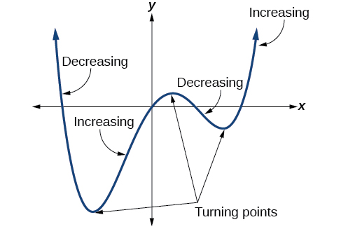
In addition to the end behavior of polynomial functions, we are also interested in what happens in the “middle” of the function. In particular, we are interested in locations where graph behavior changes. A turning point is a point at which the function values change from increasing to decreasing or decreasing to increasing.
We are also interested in the intercepts. As with all functions, the y-intercept is the point at which the graph intersects the vertical axis. The point corresponds to the coordinate pair in which the input value is zero. Because a polynomial is a function, only one output value corresponds to each input value so there can be only one y-intercept (0, a0). The x-intercepts occur at the input values that correspond to an output value of zero. It is possible to have more than one x-intercept. See the graph below.
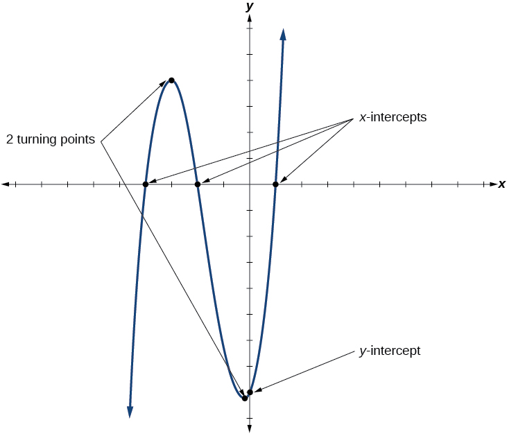
 The degree of a polynomial function helps us to determine the number of x-intercepts and the number of turning points. A polynomial function of nth degree is the product of n factors, so it will have at most n roots or zeros, or x-intercepts. The graph of the polynomial function of degree n must have at most n – 1 turning points. This means the graph has at most one fewer turning point than the degree of the polynomial or one fewer than the number of factors.
Turning Points of Polynomial Functions
A turning point of a graph is a point at which the graph changes direction from increasing to decreasing (rising to falling) or decreasing to increasing (falling to rising).
A polynomial of degree n will have at most n – 1 turning points.
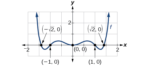
Look at the graph of the polynomial function f(x) = x4 – x3 – 4x2 + 4x below. The graph has three turning points.
This function f is a 4th degree polynomial function and has 3 turning points. The maximum number of turning points of a polynomial function is always one less than the degree of the function.
A continuous function has no breaks in its graph: the graph can be drawn without lifting the pen from the paper. A smooth curve is a graph that has no sharp corners. The turning points of a smooth graph must always occur at rounded curves. The graphs of polynomial functions are both continuous and smooth.
Try it! – Finding the Maximum Number of Turning Points Using the Degree of a Polynomial Function
Find the maximum number of turning points of each polynomial function.
- f(x) = -x3 + 4x5 – 3x2 + 1
- f(x) = -(x – 1)2(1 + 2x2)
Solution:
a. First, rewrite the polynomial function in descending order: f(x) = 4x5 – x3 – 3x2 + 1.
Identify the degree of the polynomial function. This polynomial function is of degree 5.
The maximum number of turning points is 5 – 1 = 4.
b. First, identify the leading term of the polynomial function if the function were expanded.
 Then, identify the degree of the polynomial function. This polynomial function is of degree 4. The maximum number of turning points is 4 – 1 = 3.
Finding Zeros (x-intercepts) [3]
Recall that if f is a polynomial function, the values of x for which f(x) = 0 are called zeros of f. If the equation of the polynomial function can be factored, we can set each factor equal to zero and solve for the zeros.
Zero of a Function
For any function f, if f(x) = 0, then x is a zero of the function.
When f(x) = 0, the point (x, 0) is a point on the graph. This point is an x-intercept of the graph. It is often important to know where the graph of a function crosses the axes.
Try it!
For the function f(x) = 3x2 + 10x − 8, find a. the zeros of the function, b. any x-intercepts of the graph of the function, c. any y-intercepts of the graph of the function
Solution
a. To find the zeros of the function, we need to find when the function value is 0.
| Algebraic | Steps |
| Original | f(x) = 3x2 + 10x − 8 |
| Substitute 0 for f(x). | 0 = 3x2 +10x −8 |
| Factor the trinomial. | (x + 4)(3x − 2 )= 0 |
| Use the zero product property. | x + 4x = 0 or 3x − 2x = 0 |
| Solve. | x = −4 or x = 2/3 |
b. An x-intercept occurs when y=0. Since f(−4) = 0 and f(2/3) = 0, the points (−4, 0) and (2/3, 0) lie on the graph. These points are x-intercepts of the function.
c. A y-intercept occurs when x=0. To find the y-intercepts we need to find f(0).
| Algebraic | Steps |
| Original | f(x) = 3x2 + 10x − 8 |
| Find f(0) by substituting 0 for x. | f(0) = 3 ⋅ 02 + 10 ⋅ 0 −8 |
| Simplify. | f(0) = −8 |
Since f(0) = −8, the point (0,−8) lies on the graph. This point is the y-intercept of the function.
We can use this method to find x-intercepts because at the x-intercepts we find the input values when the output value is zero. For general polynomials, this can be a challenging prospect. While quadratics can be solved using the relatively simple quadratic formula, the corresponding formulas for cubic and fourth-degree polynomials are not simple enough to remember, and formulas do not exist for general higher-degree polynomials. Consequently, we will limit ourselves to three cases:
-
- The polynomial can be factored using known methods: greatest common factor and trinomial factoring.
- The polynomial is given in factored form.
- Technology is used to determine the intercepts.
Given a polynomial function f, find the x-intercepts by factoring.
- Set f(x) = 0.
- If the polynomial function is not given in factored form:
- Factor out any common monomial factors.
- Factor any factorable binomials or trinomials.
- Set each factor equal to zero and solve to find the x-intercepts.
Try it! – Finding the x-Intercepts of a Polynomial Function by Factoring
Find the x-intercepts of f(x) = x6 – 3x4 + 2x2.
Solution:
We can attempt to factor this polynomial to find solutions for f(x) = 0.
| Steps | Algebraic |
| x6 – 3x4 + 2x4 = 0 | Factor out the greatest common factor. |
| x2(x4 – 3x2 + 2) = 0 | Factor the trinomial. |
| x2(x2 – 1)(x2 – 2) = 0 | Set each factor equal to zero. |
| (x2 – 1) = 0 | (x2 – 2) = 0 | |||
| x2 = 0 | or | x2 = 1 | or | x2 = 2 |
| x = 0 | x =  1 1 |
x =  |
This gives us five x-intercepts: (0, 0), (1, 0), (−1, 0), ( , 0), and (-, 0). See the graph below. We can see that this is an even function because it is symmetric about the y-axis.
Solution:
Find solutions for f(x) = 0 by factoring.
| Algebraic | Steps |
| x3 – 5x2 – x + 5 = 0 | Factor by grouping. |
| x2(x – 5) – 1(x – 5) = 0 | Factor out the common factor. |
| (x2 – 1)(x -5) = 0 | Factor the difference of squares. |
| (x + 1)(x – 1)(x – 5) = 0 | Set each factor equal to zero. |
| x + 1 = 0 | or | x – 1 = 0 | or | x – 5 = 0 |
| x = -1 | x = 1 | x = 5 |
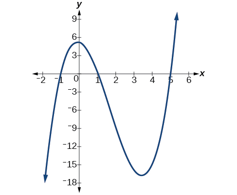
There are three x-intercepts: (-1, 0), (1, 0), and (5, 0). See the graph below.
Now that we know how to find the x-intercepts, lets combine finding both x– and y– intercepts. Remember:
Intercepts of Polynomial Functions
The y-intercept is the point at which the function has an input value of zero. The x-intercepts are the points at which the output value is zero.
- Determine the y-intercept by setting x = 0 and finding the corresponding output value.
- Determine the x-intercepts by solving for the input values that yield an output value of zero.
Try it! – Finding the y- and x-Intercepts of a Polynomial in Factored Form
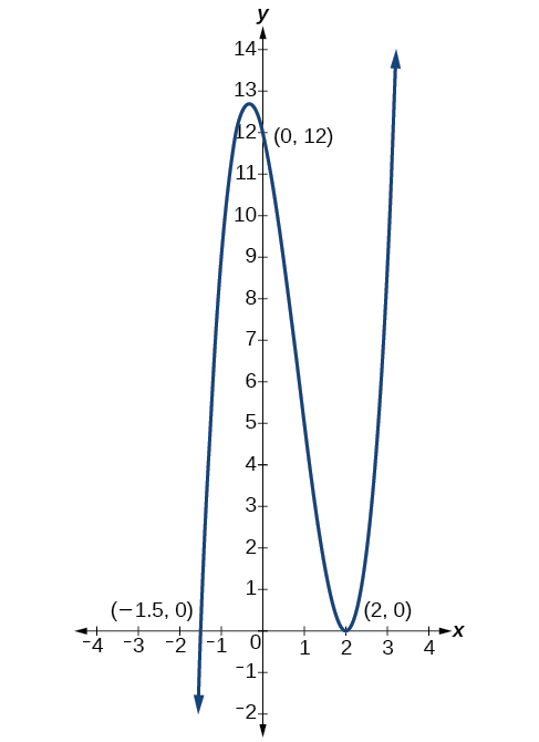
1. Find the y– and x-intercepts of g(x) = (x – 2)2(2x + 3).
Solution:
The y-intercept can be found by evaluating g(0).

So the y-intercept is (0, 12).
The x-intercepts can be found by solving g(x) = 0.
(x – 2)2(2x + 3) = 0
| (x – 2)2 = 0 | (2x + 3) = 0 | |
| x – 2 = 0 | or | x =  |
| x = 2 |
So the x-intercepts are (2, 0) and  .
.
Analysis
We can always check that our answers are reasonable by using a graphing calculator to graph the polynomial as shown below.
Solution:
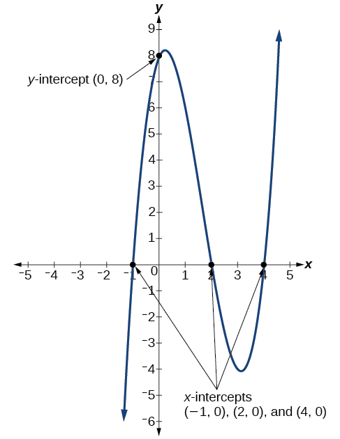
The y-intercept occurs when the input is zero so substitute 0 for x.

The y-intercept is (0, 8).
The x-intercepts occur when the output is zero.
0 = (x − 2)(x + 1) (x − 4)
| x – 2 = 0 | or | x + 1 = 0 | or | x – 4 = 0 |
| x = 2 | or | x = -1 | or | x = 4 |
The x-intercepts are (2, 0), (–1, 0), and (4, 0).
We can see these intercepts on the graph of the function shown below.
Solution:
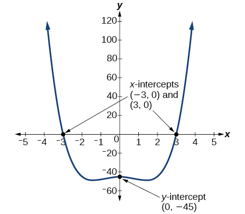
The y-intercept occurs when the input is zero.

The y-intercept is (0, −45).
The x-intercepts occur when the output is zero. To determine when the output is zero, we will need to factor the polynomial.

| x – 3 = 0 | or | x + 3 = 0 | or | x2 + 5 = 0 |
| x = 3 | or | x = -3 | or | (no real solution) |
The x-intercepts are (3, 0) and (-3, 0).
We can see these intercepts on the graph of the function shown below. We can see that the function is even because f(x) = f(-x).
4. Given the polynomial function f(x) = 2x3 – 6x2 – 20x, determine the y– and x-intercepts.
Solution:
y-intercept (0, 0); x-intercepts (0, 0), (–2, 0), and (5, 0).
Intercepts and Turning Points of Polynomials
A polynomial of degree n will have, at most, n x-intercepts and n – 1 turning points.
Try it! -Determining the Number of Intercepts and Turning Points of a Polynomial
1. Without graphing the function, determine the local behavior of the function by finding the maximum number of x-intercepts and turning points for f(x) = -3x10 + 4x7 – x4 + 2x3.
Solution:
The polynomial has a degree of 10, so there are at most 10 x-intercepts and at most 9 turning points.
2. Without graphing the function, determine the maximum number of x-intercepts and turning points for f(x) = 108 – 13x9 – 8x4 + 14x12 + 2x3.
Solution:
There are at most 12 x-intercepts and at most 11 turning points.
Try it! – Drawing Conclusions about a Polynomial Function from the Graph
1. What can we conclude about the polynomial represented by the graph shown below based on its intercepts and turning points?
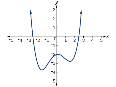
Solution:
The end behavior of the graph tells us this is the graph of an even-degree polynomial as seen below.
The graph has 2 x-intercepts, suggesting a degree of 2 or greater, and 3 turning points, suggesting a degree of 4 or greater. Based on this, it would be reasonable to conclude that the degree is even and at least 4.
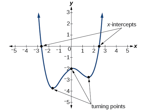
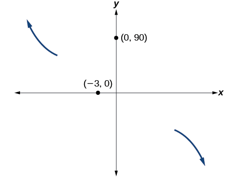
2. What can we conclude about the polynomial represented by the graph shown below based on its intercepts and turning points?
Solution:
The end behavior indicates an odd-degree polynomial function; there are 3 x-intercepts and 2 turning points, so the degree is odd and at least 3. Because of the end behavior, we know that the lead coefficient must be negative.
Try it! – Drawing Conclusions about a Polynomial Function from the Factors
Given the function f(x) = -4x(x + 3)(x – 4), determine the x– and y-intercepts, and the number of turning points.
Solution:
The y-intercept is found by evaluating f(0).

The y-intercept is (0, 0).
The x-intercepts are found by determining the zeros of the function.
0 = -4x(x + 3)(x – 4)
| -4x = 0 | or | x + 3 = 0 | or | x – 4 = 0 |
| x = 0 | or | x = -3 | or | x = 4 |
The x-intercepts are (0, 0), (-3, 0), and (4, 0).
The degree is 3 so the graph has at most 2 turning points.
Zeros and Multiplicities[4]
Graphs behave differently at various x-intercepts. Sometimes, the graph will cross over the horizontal axis at an intercept. Other times, the graph will touch the horizontal axis and “bounce” off.
Suppose, for example, we graph the function shown.
f(x) = (x + 3)(x – 2)2(x + 1)3
Notice in the graph below that the behavior of the function at each of the x-intercepts is different.
The x-intercept x = -3 is the solution of equation (x + 3) = 0. The graph passes directly through the x-intercept at x= -3. The factor is linear (has a degree of 1), so the behavior near the intercept is like that of a line—it passes directly through the intercept. We call this a single zero because the zero corresponds to a single factor of the function.
The x-intercept x = 2 is the repeated solution of equation (x – 2)2 = 0. The graph touches the axis at the intercept and changes direction. The factor is quadratic (degree 2), so the behavior near the intercept is like that of a quadratic—it bounces off of the horizontal axis at the intercept.
(x – 2)2 = (x – 2)(x – 2)
The factor is repeated, that is, the factor (x − 2) appears twice. The number of times a given factor appears in the factored form of the equation of a polynomial is called the multiplicity. The zero associated with this factor, x = 2, has multiplicity 2 because the factor (x – 2) occurs twice.
The x-intercept x = -1 is the repeated solution of factor (x + 1)3 = 0. The graph passes through the axis at the intercept, but flattens out a bit first. This factor is cubic (degree 3), so the behavior near the intercept is like that of a cubic—with the same S-shape near the intercept as the toolkit function f(x) = x3. We call this a triple zero, or a zero with multiplicity 3.
For zeros with even multiplicities, the graphs touch or are tangent to the x-axis. For zeros with odd multiplicities, the graphs cross or intersect the x-axis. See the figure below for examples of graphs of polynomial functions with multiplicity 1, 2, and 3.
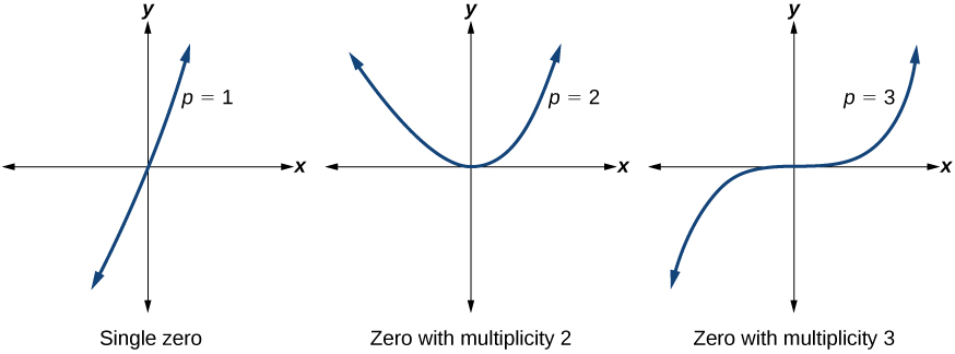
For higher even powers, such as 4, 6, and 8, the graph will still touch and bounce off of the horizontal axis but, for each increasing even power, the graph will appear flatter as it approaches and leaves the x-axis.
For higher odd powers, such as 5, 7, and 9, the graph will still cross through the horizontal axis, but for each increasing odd power, the graph will appear flatter as it approaches and leaves the x-axis.
Graphical Behavior of Polynomials at x-Intercepts
If a polynomial contains a factor of the form (x – h)p, the behavior near the x-intercept h is determined by the power p. We say that x = h is a zero of multiplicity p.
The graph of a polynomial function will touch the x-axis at zeros with even multiplicities. The graph will cross the x-axis at zeros with odd multiplicities.
The sum of the multiplicities is the degree of the polynomial function.
How to identify the zeros and their multiplicities from a graph of a polynomial function of degree n.
- If the graph crosses the x-axis and appears almost linear at the intercept, it is a single zero.
- If the graph touches the x-axis and bounces off of the axis, it is a zero with even multiplicity.
- If the graph crosses the x-axis at a zero, it is a zero with odd multiplicity.
- The sum of the multiplicities is n.
Try it! – Identifying Zeros and Their Multiplicities
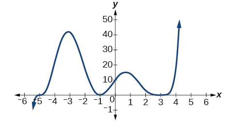
1. Use the graph of the function of degree 6 below to identify the zeros of the function and their possible multiplicities.
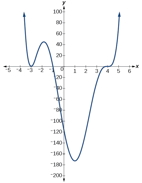
Solution:
The polynomial function is of degree 6. The sum of the multiplicities must be 6.
Starting from the left, the first zero occurs at x = -3. The graph touches the x-axis, so the multiplicity of the zero must be even. The zero of -3 most likely has multiplicity 2.
The next zero occurs at x = -1. The graph looks almost linear at this point. This is a single zero of multiplicity 1.
The last zero occurs at x = 4. The graph crosses the x-axis, so the multiplicity of the zero must be odd. We know that the multiplicity is likely 3 and that the sum of the multiplicities is 6.
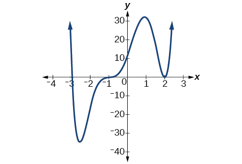
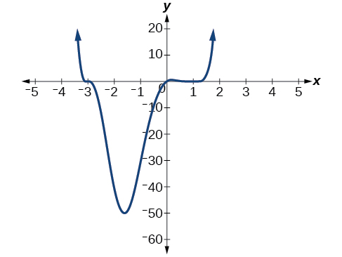
2. Use the graph of the function of degree 9 below to identify the zeros of the function and their multiplicities.
Solution:
The graph has a zero of –5 with multiplicity 3, a zero of -1 with multiplicity 2, and a zero of 3 with multiplicity 4.
Graphing Polynomial Functions[5]
We can use what we have learned about multiplicities, end behavior, and turning points to sketch graphs of polynomial functions. Let us put this all together and look at the steps required to graph polynomial functions.
How to sketch the graph of a polynomial function.
- Find the intercepts.
- Check for symmetry. If the function is an even function, its graph is symmetrical about the y-axis, that is, f(−x) = f(x). If a function is an odd function, its graph is symmetrical about the origin, that is, f(-x) = -f(x).
- Use the multiplicities of the zeros to determine the behavior of the polynomial at the x-intercepts.
- Determine the end behavior by examining the leading term.
- Use the end behavior and the behavior at the intercepts to sketch a graph.
- Ensure that the number of turning points does not exceed one less than the degree of the polynomial.
- Optionally, use technology to check the graph.
Try it! – Sketching the Graph of a Polynomial Function
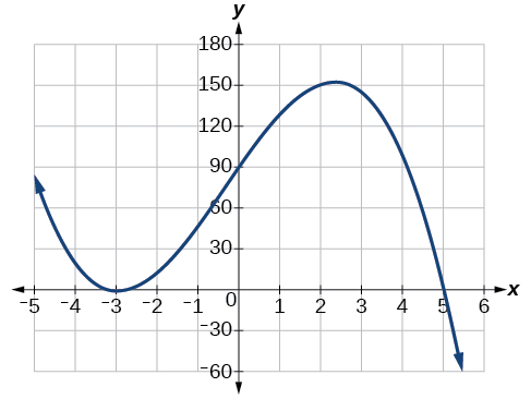
1. Sketch a graph of f(x) = -2(x + 3)2(x − 5).
Solution:
This graph has two x-intercepts. At x = −3, the factor is squared, indicating a multiplicity of 2. The graph will bounce at this x-intercept. At x = 5, the function has a multiplicity of one, indicating the graph will cross through the axis at this intercept.
The y-intercept is found by evaluating f(0).

The y-intercept is (0, 90).
Additionally, we can see the leading term, if this polynomial were multiplied out, would be -2x3, so the end behavior is that of a vertically reflected cubic, with the outputs decreasing as the inputs approach infinity, and the outputs increasing as the inputs approach negative infinity. See the graph below.

To sketch this, we consider that:
- As x → −∞ the function f(x) → ∞, so we know the graph starts in the second quadrant and is decreasing toward the x-axis.
- Since f(−x) = -2(−x + 3)2(-x – 5) is not equal to f(x), the graph does not display symmetry.
- At (−3, 0), the graph bounces off of the x-axis, so the function must start increasing.
At (0, 90), the graph crosses the y-axis at the y-intercept. See the graph below.
Somewhere after this point, the graph must turn back down or start decreasing toward the horizontal axis because the graph passes through the next intercept at (5, 0). See the graph below.

As x → ∞ the function f(x) → −∞, so we know the graph continues to decrease, and we can stop drawing the graph in the fourth quadrant.
Using technology, we can create the graph for the polynomial function, shown in the graph below, and verify that the resulting graph looks like our sketch in the graph above.
2. Sketch a graph of  .
.
Solution:
Intermediate Value Theorem[6]
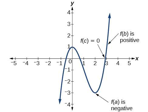
In some situations, we may know two points on a graph but not the zeros. If those two points are on opposite sides of the x-axis, we can confirm that there is a zero between them. Consider a polynomial function f whose graph is smooth and continuous. The Intermediate Value Theorem states that for two numbers a and b in the domain of f, if a < b and f(a) ≠ f(b), then the function f takes on every value between f(a) and f(b). (While the theorem is intuitive, the proof is actually quite complicated and requires higher mathematics). We can apply this theorem to a special case that is useful in graphing polynomial functions. If a point on the graph of a continuous function f at x = a lies above the x-axis and another point at x = b lies below the x-axis, there must exist a third point between x = a and x = b where the graph crosses the x-axis. Call this point (c, f(c)). This means that we are assured there is a solution c where f(c) = 0.
In other words, the Intermediate Value Theorem tells us that when a polynomial function changes from a negative value to a positive value, the function must cross the x-axis. The figure below shows that there is a zero between a and b.
Intermediate Value Theorem
Let f be a polynomial function. The Intermediate Value Theorem states that if f(a) and f(b) have opposite signs, then there exists at least one value c between a and b for which f(c) = 0.
Try it! – Using the Intermediate Value Theorem
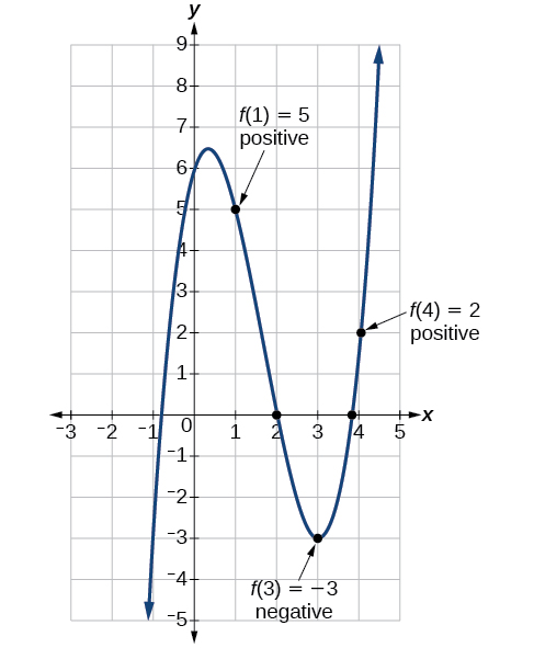
1. Show that the function f(x) = x3 – 5x2 + 3x + 6 has at least two real zeros between x = 1 and x = 4.
Solution:
As a start, evaluate f(x) at the integer values x = 1, 2, 3, and 4. See the table below.
| Solution | ||||
| x | 1 | 2 | 3 | 4 |
| f(x) | 5 | 0 | –3 | 2 |
We see that one zero occurs at x = 2. Also, since f(3) is negative and f(4) is positive, by the Intermediate Value Theorem, there must be at least one real zero between 3 and 4.
We have shown that there are at least two real zeros between x = 1 and x = 4.
Analysis
We can also see on the graph of the function below that there are two real zeros between x = 1 and x = 4.
2. Show that the function f(x) = 7x5 – 9x4 – x2 has at least one real zero between x = 1 and x = 2.
Solution:
Because f is a polynomial function and since f(1) is negative and f(2)is positive, there is at least one real zero between x = 1 and x = 2.
Access these online resources for additional instruction and practice with power and polynomial functions.
Key Concepts
- Polynomials
- Polynomial—A monomial, or two or more algebraic terms combined by addition or subtraction is a polynomial.
- monomial —A polynomial with exactly one term is called a monomial.
- binomial — A polynomial with exactly two terms is called a binomial.
- trinomial —A polynomial with exactly three terms is called a trinomial.
- Degree of a Polynomial
- The degree of a term is the sum of the exponents of its variables.
- The degree of a constant is 0.
- The degree of a polynomial is the highest degree of all its terms.
- The behavior of a graph as the input decreases beyond bound and increases beyond bound is called the end behavior.
- The end behavior depends on whether the power is even or odd.
- A polynomial function is the sum of terms, each of which consists of a transformed power function with positive whole number power.
- The degree of a polynomial function is the highest power of the variable that occurs in a polynomial. The term containing the highest power of the variable is called the leading term. The coefficient of the leading term is called the leading coefficient.
- The end behavior of a polynomial function is the same as the end behavior of the power function represented by the leading term of the function.
- Polynomial functions of degree 2 or more are smooth, continuous functions.
- To find the zeros of a polynomial function, if it can be factored, factor the function and set each factor equal to zero.
- Another way to find the x-intercepts of a polynomial function is to graph the function and identify the points at which the graph crosses the x-axis.
- The multiplicity of a zero determines how the graph behaves at the x-intercepts.
- The graph of a polynomial will cross the horizontal axis at a zero with odd multiplicity.
- The graph of a polynomial will touch the horizontal axis at a zero with even multiplicity.
- The end behavior of a polynomial function depends on the leading term.
- The graph of a polynomial function changes direction at its turning points.
- A polynomial function of degree n has at most n – 1 turning points.
- To graph polynomial functions, find the zeros and their multiplicities, determine the end behavior, and ensure that the final graph has at most n – 1 turning points.
- The Intermediate Value Theorem tells us that if f(a) and f(b) have opposite signs, then there exists at least one value c between a and b for which f(c) = 0.
- Access for free at https://openstax.org/books/intermediate-algebra-2e/pages/1-introduction, derived from Add and subtract polynomials. Also Access for free at https://openstax.org/books/college-algebra-corequisite-support-2e/pages/1-introduction-to-prerequisites, Power functions and polynomial functions and Graphs of Polynomial functions ↵
- Access for free at https://openstax.org/books/college-algebra-corequisite-support-2e/pages/1-introduction-to-prerequisites, Power functions and polynomial functions and Graphs of Polynomial functions ↵
- Access for free at https://openstax.org/books/intermediate-algebra-2e/pages/1-introduction, Polynomial Equations. Also Access for free at https://openstax.org/books/college-algebra-corequisite-support-2e/pages/1-introduction-to-prerequisites, Graphs of Polynomial functions ↵
- Access for free at https://openstax.org/books/college-algebra-corequisite-support-2e/pages/1-introduction-to-prerequisites, Graphs of Polynomial functions ↵
- Access for free at https://openstax.org/books/college-algebra-corequisite-support-2e/pages/1-introduction-to-prerequisites, Graphs of Polynomial functions ↵
- Access for free at https://openstax.org/books/college-algebra-corequisite-support-2e/pages/1-introduction-to-prerequisites, Graphs of Polynomial functions ↵
A monomial or two or more monomials combined by addition or subtraction is a polynomial.
A monomial is an algebraic expression with one term. A monomial in one variable is a term of the form [latex]ax^m[/latex], where a is a constant and m is a whole number.
A binomial is a polynomial with exactly two terms.
A trinomial is a polynomial with exactly three terms.
The degree of a term is the sum of the exponents of its variables.
The degree of any constant is 0.
The degree of a polynomial is the highest degree of all its terms
A polynomial is in standard form when the terms of a polynomial are written in descending order of degrees.
A polynomial function is a function whose range values are defined by a polynomial.
A value of x where the function is 0, is called a zero of the function.
